Main Content

Visualize PDE Results

Create and explore visualizations of PDE results in the Live Editor

Since R2022b

Description

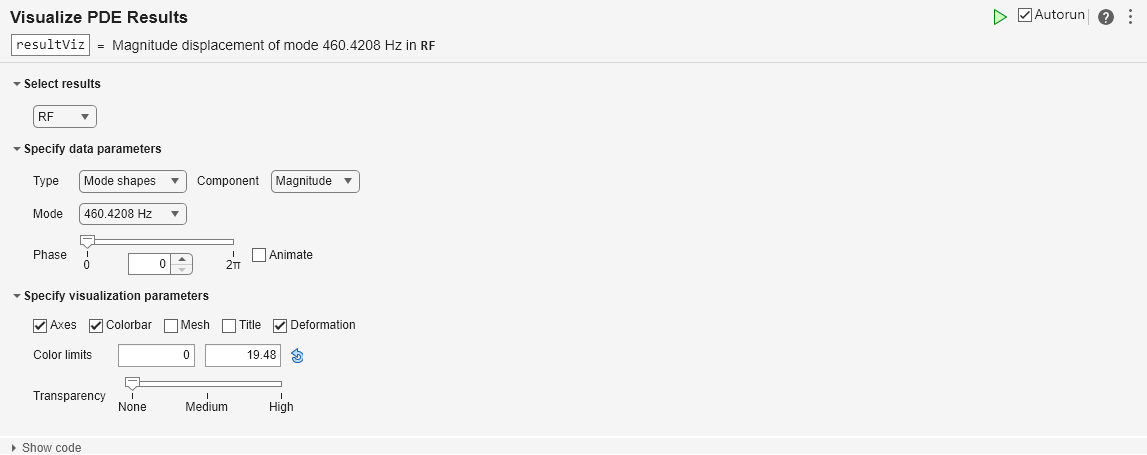
The Visualize PDE Results task enables you to plot and inspect results of structural, thermal, electromagnetic, or general PDE analysis using interactive controls. The task automatically generates MATLAB® code for your live script.

Using this task, you can:

  • Select which solution data to display.

  • Quickly access plots for different frequencies, modes, time steps, and phases.

  • Show animated solutions.

  • Add a mesh to a solution plot.

  • Adjust color limits for a colormap.

  • Adjust surface transparency.

For general information about Live Editor tasks, see Add Interactive Tasks to a Live Script.

Visualize PDE Results task in the Live Editor

Open the Task

To add the Visualize PDE Results task to a live script in the MATLAB Editor:

  • On the Live Editor tab, select Task > Visualize PDE Results.

  • In a code block in the script, type a relevant keyword, such as pde. Select Visualize PDE Results from the suggested command completions.

Examples

expand all

Use the Visualize PDE Results task in the Live Editor to explore structural modal analysis results of a tuning fork. Open this example to see a preconfigured script containing the Visualize PDE Results task.

Find natural frequencies and mode shapes for the fundamental mode of a tuning fork and the next several modes. To perform unconstrained modal analysis of a structure, you can specify just the geometry, mesh, and material properties.

model = createpde("structural","modal-solid");
importGeometry(model,"TuningFork.stl");
structuralProperties(model,"YoungsModulus",210e9, ...
                           "PoissonsRatio",0.3, ...
                           "MassDensity",8000);
generateMesh(model,"Hmax",0.001);

Solve the model for a chosen frequency range.

RF = solve(model,"FrequencyRange",[-1,4000]*2*pi);

To visualize mode shapes, open the Visualize PDE Results Live Editor task. On the Live Editor tab, select Task > Visualize PDE Results. This action inserts the task into your script.

Live Task

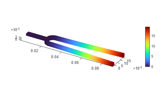
In the Select results section of the task, select RF from the drop-down list. Because there are no boundary constraints in this example, modal results include the rigid body modes. The first six near-zero frequencies indicate the six rigid body modes of the 3-D tuning fork. The first flexible mode is the seventh mode with a frequency of about 460 Hz.

Live Task

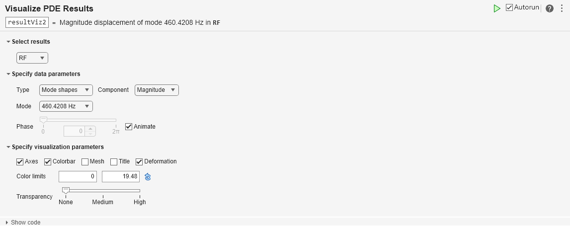
The best way to visualize mode shapes is to animate the harmonic motion at their respective frequencies. Select Animate to see the harmonic motion at a frequency of about 460 Hz.

Live Task

Related Examples

Parameters

expand all

Choose the results to plot from the structural, thermal, electromagnetic, and general PDE results available in the MATLAB workspace. You can select only one solution at a time. The solution must be specified as one of these objects:

Specify data parameters

Choose the part of the solution to plot, such as a displacement for a structural problem, temperature for a thermal problem, or electric field for an electrostatic problem.

Choose to plot the x-, y-, or z-component of a solution such as displacement, stress, temperature gradient, electric field, or magnetic field.

Choose the number corresponding to the solution mode to plot.

Choose the number corresponding to the solution frequency to plot.

Choose the number corresponding to the eigenvalue of a thermal model.

Choose the number corresponding to the equation to plot.

Choose the number corresponding to the eigenvalue of a PDE model.

Choose the time to plot results for. The slider values correspond to the times that you used when solving the problem.

Choose the phase to plot results for. The slider values are from 0 to 2π.

Select this option to play the animation.

Specify visualization parameters

Select this option to show the coordinate axes.

Select this option to show the color bar.

Select this option to show the mesh.

Select this option to show an autogenerated plot title.

Switch between deformed and undeformed shapes for a 3-D structural model. In an undeformed shape, center nodes in quadratic meshes are always added at the halfway point between corners. When you plot a deformed shape, the center nodes can move away from the edge centers.

Set the colormap limits. The default mapping is useful in most cases, but you can perform the mapping over any range you choose, even if the range you choose is different than the range of your data. Choosing a different mapping range allows you to:

  • See where your data is at or beyond the limits of that range.

  • See where your data lies within that range.

For details, see Control Colormap Limits.

Adjust the surface transparency by moving the slider between None, Medium, and High.

Version History

Introduced in R2022b