Semantic Segmentation Using Deep Learning

Download Pretrained Semantic Segmentation Network

Download a pretrained version of DeepLab v3+ trained on the CamVid dataset.

pretrainedURL = "https://ssd.mathworks.com/supportfiles/vision/data/deeplabv3plusResnet18CamVid_v2.zip";
pretrainedFolder = fullfile(tempdir,"pretrainedNetwork");
pretrainedNetworkZip = fullfile(pretrainedFolder,"deeplabv3plusResnet18CamVid_v2.zip"); 
if ~exist(pretrainedNetworkZip,'file')
    mkdir(pretrainedFolder);
    disp("Downloading pretrained network (58 MB)...");
    websave(pretrainedNetworkZip,pretrainedURL);
end

Downloading pretrained network (58 MB)...

unzip(pretrainedNetworkZip, pretrainedFolder)

Load the pretrained network.

pretrainedNetwork = fullfile(pretrainedFolder,"deeplabv3plusResnet18CamVid_v2.mat");  
data = load(pretrainedNetwork);
net = data.net;

Set the classes this network has been trained to classify.

classes = getClassNames()

classes = 11×1 string
    "Sky"
    "Building"
    "Pole"
    "Road"
    "Pavement"
    "Tree"
    "SignSymbol"
    "Fence"
    "Car"
    "Pedestrian"
    "Bicyclist"

Perform Semantic Image Segmentation

Read an image that contains classes the network is trained to classify.

I = imread("parkinglot_left.png");

Resize the image to the input size of the network.

inputSize = net.Layers(1).InputSize;
I = imresize(I,inputSize(1:2));

Perform semantic segmentation using the semanticseg function and the pretrained network.

C = semanticseg(I,net);

Overlay the segmentation results on top of the image with labeloverlay. Set the overlay color map to the color map values defined by the CamVid dataset [2].

cmap = camvidColorMap;
B = labeloverlay(I,C,Colormap=cmap,Transparency=0.4);
figure
imshow(B)
pixelLabelColorbar(cmap, classes);

Although the network is pretrained on images of city driving, it produces a reasonable result on a parking lot scene. To improve the segmentation results, the network should be retrained with additional images that contain parking lot scenes. The remainder of this example shows you how to train a semantic segmentation network using transfer learning.

Train a Semantic Segmentation Network

This example trains a Deeplab v3+ network with weights initialized from a pre-trained Resnet-18 network. ResNet-18 is an efficient network that is well suited for applications with limited processing resources. Other pretrained networks such as MobileNet v2 or ResNet-50 can also be used depending on application requirements. For more details, see Pretrained Deep Neural Networks (Deep Learning Toolbox).

Get a pretrained ResNet-18 network using the imagePretrainedNetwork function. ResNet-18 requires the Deep Learning Toolbox™ Model for ResNet-18 Network support package. If this support package is not installed, then the function provides a download link.

imagePretrainedNetwork("resnet18")

ans = 
  dlnetwork with properties:

         Layers: [70×1 nnet.cnn.layer.Layer]
    Connections: [77×2 table]
     Learnables: [82×3 table]
          State: [40×3 table]
     InputNames: {'data'}
    OutputNames: {'prob'}
    Initialized: 1

  View summary with summary.

Download CamVid Dataset

Download the CamVid dataset from the following URLs.

imageURL = "http://web4.cs.ucl.ac.uk/staff/g.brostow/MotionSegRecData/files/701_StillsRaw_full.zip";
labelURL = "http://web4.cs.ucl.ac.uk/staff/g.brostow/MotionSegRecData/data/LabeledApproved_full.zip";
 
outputFolder = fullfile(tempdir,"CamVid"); 
labelsZip = fullfile(outputFolder,"labels.zip");
imagesZip = fullfile(outputFolder,"images.zip");

if ~exist(labelsZip, 'file') || ~exist(imagesZip,'file')   
    mkdir(outputFolder)
       
    disp("Downloading 16 MB CamVid dataset labels..."); 
    websave(labelsZip, labelURL);
    unzip(labelsZip, fullfile(outputFolder,"labels"));
    
    disp("Downloading 557 MB CamVid dataset images...");  
    websave(imagesZip, imageURL);       
    unzip(imagesZip, fullfile(outputFolder,"images"));    
end

Downloading 16 MB CamVid dataset labels...

Downloading 557 MB CamVid dataset images...

Note: Download time of the data depends on your Internet connection. The commands used above block MATLAB until the download is complete. Alternatively, you can use your web browser to first download the dataset to your local disk. To use the file you downloaded from the web, change the outputFolder variable above to the location of the downloaded file.

Load CamVid Images

Use imageDatastore to load CamVid images. The imageDatastore enables you to efficiently load a large collection of images on disk.

imgDir = fullfile(outputFolder,"images","701_StillsRaw_full");
imds = imageDatastore(imgDir);

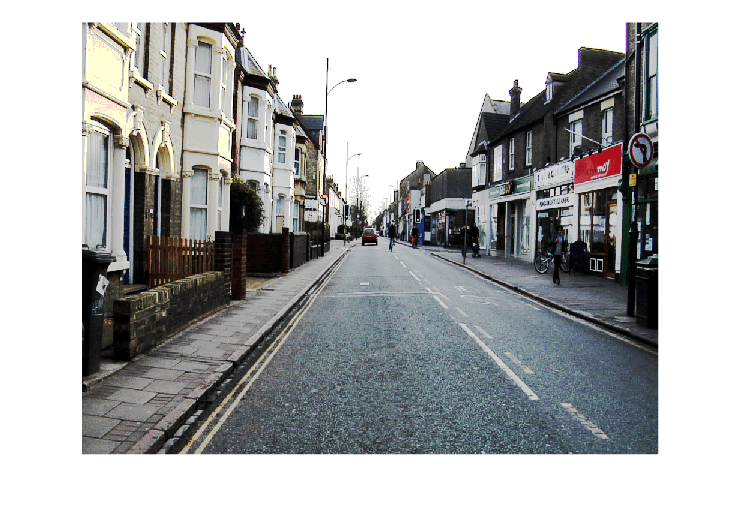
Display one of the images.

I = readimage(imds,559);
I = histeq(I);
imshow(I)

Load CamVid Pixel-Labeled Images

Use pixelLabelDatastore to load CamVid pixel label image data. A pixelLabelDatastore encapsulates the pixel label data and the label ID to a class name mapping.

To make training easier, group the 32 original classes in CamVid to 11 classes. To reduce 32 classes into 11, multiple classes from the original dataset are grouped together. For example, "Car" is a combination of "Car", "SUVPickupTruck", "Truck_Bus", "Train", and "OtherMoving". Return the grouped label IDs by using the supporting function camvidPixelLabelIDs, which is listed at the end of this example.

labelIDs = camvidPixelLabelIDs();

Use the classes and label IDs to create the pixelLabelDatastore.

labelDir = fullfile(outputFolder,"labels");
pxds = pixelLabelDatastore(labelDir,classes,labelIDs);

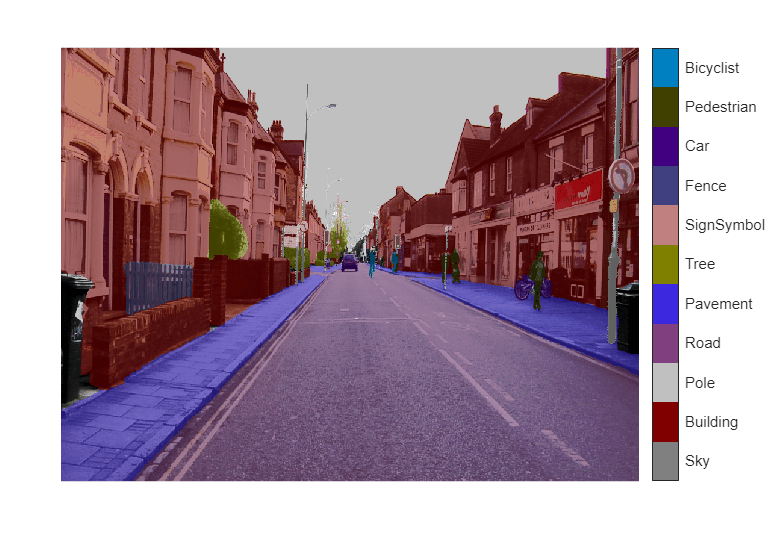
Read and display one of the pixel-labeled images by overlaying it on top of an image. Areas with no color overlay do not have pixel labels and are not used during training.

C = readimage(pxds,559);
cmap = camvidColorMap;
B = labeloverlay(I,C,ColorMap=cmap);
imshow(B)
pixelLabelColorbar(cmap,classes);

Analyze Dataset Statistics

To see the distribution of class labels in the CamVid dataset, use countEachLabel. This function counts the number of pixels by class label.

tbl = countEachLabel(pxds)

tbl=11×3 table
         Name         PixelCount    ImagePixelCount
    ______________    __________    _______________

    {'Sky'       }    7.6801e+07      4.8315e+08   
    {'Building'  }    1.1737e+08      4.8315e+08   
    {'Pole'      }    4.7987e+06      4.8315e+08   
    {'Road'      }    1.4054e+08      4.8453e+08   
    {'Pavement'  }    3.3614e+07      4.7209e+08   
    {'Tree'      }    5.4259e+07       4.479e+08   
    {'SignSymbol'}    5.2242e+06      4.6863e+08   
    {'Fence'     }    6.9211e+06       2.516e+08   
    {'Car'       }    2.4437e+07      4.8315e+08   
    {'Pedestrian'}    3.4029e+06      4.4444e+08   
    {'Bicyclist' }    2.5912e+06      2.6196e+08   

Visualize the pixel counts by class.

frequency = tbl.PixelCount/sum(tbl.PixelCount);

bar(1:numel(classes),frequency)
xticks(1:numel(classes)) 
xticklabels(tbl.Name)
xtickangle(45)
ylabel("Frequency")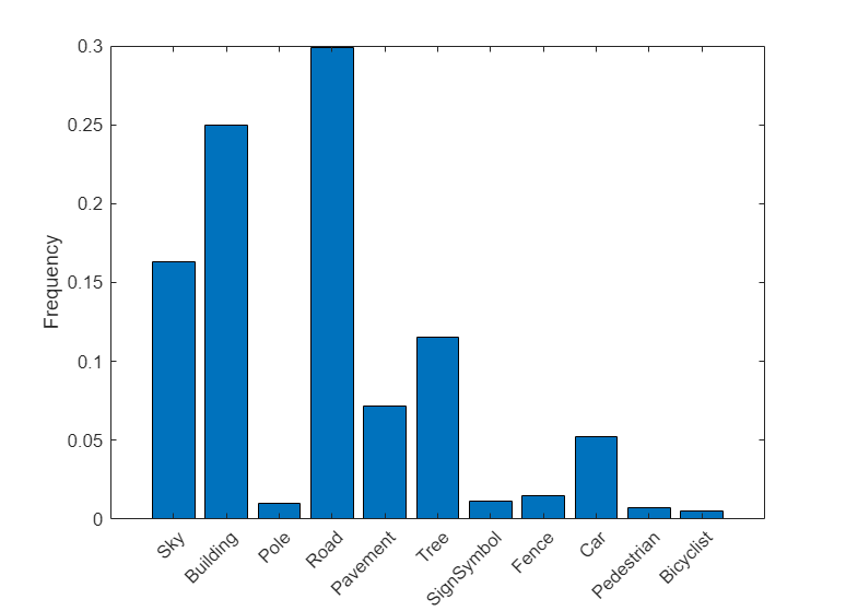

Ideally, all classes would have an equal number of observations. However, the classes in CamVid are imbalanced, which is a common issue in automotive data-sets of street scenes. Such scenes have more sky, building, and road pixels than pedestrian and bicyclist pixels because sky, buildings and roads cover more area in the image. If not handled correctly, this imbalance can be detrimental to the learning process because the learning is biased in favor of the dominant classes. Later on in this example, you will use class weighting to handle this issue.

Prepare Training, Validation, and Test Sets

Deeplab v3+ is trained using 60% of the images from the dataset. The rest of the images are split evenly in 20% and 20% for validation and testing respectively. The following code randomly splits the image and pixel label data into a training, validation and test set.

[imdsTrain, imdsVal, imdsTest, pxdsTrain, pxdsVal, pxdsTest] = partitionCamVidData(imds,pxds);

The 60/20/20 split results in the following number of training, validation and test images:

numTrainingImages = numel(imdsTrain.Files)

numTrainingImages = 421

numValImages = numel(imdsVal.Files)

numValImages = 140

numTestingImages = numel(imdsTest.Files)

numTestingImages = 140

Define validation data.

dsVal = combine(imdsVal,pxdsVal);

Data Augmentation

Data augmentation is used to improve network accuracy by randomly transforming the original data during training. By using data augmentation, you can add more variety to the training data without increasing the number of labeled training samples. To apply the same random transformation to both image and pixel label data use datastore combine and transform. First, combine imdsTrain and pxdsTrain.

dsTrain = combine(imdsTrain,pxdsTrain);

Next, use datastore transform to apply the desired data augmentation defined in the supporting function augmentImageAndLabel. Here, random left/right reflection and random X/Y translation of +/- 10 pixels is used for data augmentation.

xTrans = [-10 10];
yTrans = [-10 10];
dsTrain = transform(dsTrain, @(data)augmentImageAndLabel(data,xTrans,yTrans));

Note that data augmentation is not applied to the test and validation data. Ideally, test and validation data should be representative of the original data and is left unmodified for unbiased evaluation.

Create the Network

Specify the network image size. This is typically the same as the training image sizes.

imageSize = [720 960 3];

Specify the number of classes.

numClasses = numel(classes);

Use the deeplabv3plus function to create a DeepLab v3+ network based on ResNet-18. Choosing the best network for your application requires empirical analysis and is another level of hyperparameter tuning. For example, you can experiment with different base networks such as ResNet-50 or MobileNet v2, or you can try another semantic segmentation network architecture such as U-Net.

network = deeplabv3plus(imageSize,numClasses,"resnet18");

Balance Classes Using Class Weighting

As shown earlier, the classes in CamVid are not balanced. To improve training, you can use class weighting to balance the classes. Use the pixel label counts computed earlier with the countEachLabel function and calculate the median frequency class weights.

imageFreq = tbl.PixelCount ./ tbl.ImagePixelCount;
classWeights = median(imageFreq) ./ imageFreq;

Select Training Options

The optimization algorithm used for training is stochastic gradient descent with momentum (SGDM). Use trainingOptions (Deep Learning Toolbox) to specify the hyper-parameters used for SGDM.

The learning rate uses a piecewise schedule. The learning rate is reduced by a factor of 0.1 every 6 epochs. This allows the network to learn quickly with a higher initial learning rate, while being able to find a solution close to the local optimum once the learning rate drops.

The network is tested against the validation data every epoch by setting the ValidationData name-value argument. The ValidationPatience is set to 4 to stop training early when the validation accuracy converges. This prevents the network from overfitting on the training dataset.

A mini-batch size of 4 is used to reduce memory usage while training. You can increase or decrease this value based on the amount of GPU memory you have on your system.

In addition, CheckpointPath is set to a temporary location. This name-value argument enables the saving of network checkpoints at the end of every training epoch. If training is interrupted due to a system failure or power outage, you can resume training from the saved checkpoint. Make sure that the location specified by CheckpointPath has enough space to store the network checkpoints. For example, saving 100 Deeplab v3+ checkpoints requires ~6 GB of disk space because each checkpoint is 61 MB.

options = trainingOptions("sgdm",...
    LearnRateSchedule="piecewise",...
    LearnRateDropPeriod=6,...
    LearnRateDropFactor=0.1,...
    Momentum=0.9,...
    InitialLearnRate=1e-2,...
    L2Regularization=0.005,...
    ValidationData=dsVal,...
    MaxEpochs=18,...  
    MiniBatchSize=4,...
    Shuffle="every-epoch",...
    CheckpointPath=tempdir,...
    VerboseFrequency=10,...
    ValidationPatience=4);

Start Training

To train the network, set the doTraining variable in the following code to true. Train the neural network using the trainnet (Deep Learning Toolbox) function. Use a custom loss function, specified by the modelLoss helper function. By default, the trainnet function uses a GPU if one is available. Training on a GPU requires a Parallel Computing Toolbox™ license and a supported GPU device. For information on supported devices, see GPU Computing Requirements (Parallel Computing Toolbox). Otherwise, the trainnet function uses the CPU. To specify the execution environment, use the ExecutionEnvironment training option.

Note: The training was verified on an NVIDIA™ GeForce RTX 3090 Ti with 24 GB of memory. If your GPU has less memory, you may run out of memory during training. If this happens, try setting MiniBatchSize to 1 in trainingOptions, or reducing the network input size and resizing the training data. Training this network takes about 50 minutes. Depending on your GPU hardware, it may take longer.

doTraining = false;
if doTraining
    [net,info] = trainnet(dsTrain,network,@(Y,T) modelLoss(Y,T,classWeights),options);
end

Test Network on One Image

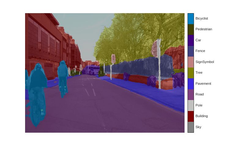
Run the trained network on one test image.

I = readimage(imdsTest,35);
C = semanticseg(I,net,Classes=classes);

Display the results.

B = labeloverlay(I,C,Colormap=cmap,Transparency=0.4);
imshow(B)
pixelLabelColorbar(cmap, classes);

Compare the results in C with the expected ground truth stored in pxdsTest. The green and magenta regions highlight areas where the segmentation results differ from the expected ground truth.

expectedResult = readimage(pxdsTest,35);
actual = uint8(C);
expected = uint8(expectedResult);
imshowpair(actual, expected)

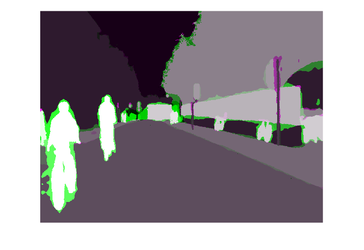
Visually, the semantic segmentation results overlap well for classes such as road, sky, tree, and building. However, smaller objects like pedestrians and cars are not as accurate. The amount of overlap per class can be measured using the intersection-over-union (IoU) metric, also known as the Jaccard index. Use the jaccard function to measure IoU.

iou = jaccard(C,expectedResult);
table(classes,iou)

ans=11×2 table
      classes         iou  
    ____________    _______

    "Sky"           0.93632
    "Building"      0.87723
    "Pole"          0.40475
    "Road"          0.95332
    "Pavement"       0.8558
    "Tree"          0.92632
    "SignSymbol"    0.62978
    "Fence"         0.82389
    "Car"           0.75381
    "Pedestrian"    0.26717
    "Bicyclist"      0.7058

The IoU metric confirms the visual results. Road, sky, tree, and building classes have high IoU scores, while classes such as pedestrian and car have low scores. Other common segmentation metrics include the dice and the bfscore contour matching score.

Evaluate Trained Network

To measure accuracy for multiple test images, runsemanticseg on the entire test set. A mini-batch size of 4 is used to reduce memory usage while segmenting images. You can increase or decrease this value based on the amount of GPU memory you have on your system.

pxdsResults = semanticseg(imdsTest,net, ...
    Classes=classes, ...
    MiniBatchSize=4, ...
    WriteLocation=tempdir, ...
    Verbose=false);

semanticseg returns the results for the test set as a pixelLabelDatastore object. The actual pixel label data for each test image in imdsTest is written to disk in the location specified by the WriteLocation name-value argument. UseevaluateSemanticSegmentation to measure semantic segmentation metrics on the test set results.

metrics = evaluateSemanticSegmentation(pxdsResults,pxdsTest,Verbose=false);

evaluateSemanticSegmentation returns various metrics for the entire dataset, for individual classes, and for each test image. To see the dataset level metrics, inspect metrics.DataSetMetrics. The dataset metrics provide a high-level overview of the network performance.

metrics.DataSetMetrics

ans=1×5 table
    GlobalAccuracy    MeanAccuracy    MeanIoU    WeightedIoU    MeanBFScore
    ______________    ____________    _______    ___________    ___________

       0.90748          0.88828       0.69573      0.84904        0.74304  

To see the impact each class has on the overall performance, inspect the per-class metrics using metrics.ClassMetrics.

Although the overall dataset performance is quite high, the class metrics show that underrepresented classes such as Pedestrian, Bicyclist, and Car are not segmented as well as classes such as Road, Sky, Tree, and Building. Additional data that includes more samples of the underrepresented classes might help improve the results.

metrics.ClassMetrics

ans=11×3 table
                  Accuracy      IoU      MeanBFScore
                  ________    _______    ___________

    Sky            0.9438     0.91456      0.91326  
    Building      0.84484     0.82403      0.69502  
    Pole          0.82513     0.29465      0.65171  
    Road          0.94803     0.93847      0.84376  
    Pavement      0.92135     0.77639      0.80391  
    Tree          0.89106     0.79122      0.76429  
    SignSymbol    0.81774     0.49374       0.5954  
    Fence         0.81991      0.6213      0.63421  
    Car           0.93654      0.8163       0.7784  
    Pedestrian    0.91095     0.50498      0.69317  
    Bicyclist     0.91172     0.67738      0.72119  

Supporting Functions

function labelIDs = camvidPixelLabelIDs()
% Return the label IDs corresponding to each class.
%
% The CamVid dataset has 32 classes. Group them into 11 classes following
% the original SegNet training methodology [1].
%
% The 11 classes are:
%   "Sky" "Building", "Pole", "Road", "Pavement", "Tree", "SignSymbol",
%   "Fence", "Car", "Pedestrian",  and "Bicyclist".
%
% CamVid pixel label IDs are provided as RGB color values. Group them into
% 11 classes and return them as a cell array of M-by-3 matrices. The
% original CamVid class names are listed alongside each RGB value. Note
% that the Other/Void class are excluded below.
labelIDs = { ...
    
    % "Sky"
    [
    128 128 128; ... % "Sky"
    ]
    
    % "Building" 
    [
    000 128 064; ... % "Bridge"
    128 000 000; ... % "Building"
    064 192 000; ... % "Wall"
    064 000 064; ... % "Tunnel"
    192 000 128; ... % "Archway"
    ]
    
    % "Pole"
    [
    192 192 128; ... % "Column_Pole"
    000 000 064; ... % "TrafficCone"
    ]
    
    % Road
    [
    128 064 128; ... % "Road"
    128 000 192; ... % "LaneMkgsDriv"
    192 000 064; ... % "LaneMkgsNonDriv"
    ]
    
    % "Pavement"
    [
    000 000 192; ... % "Sidewalk" 
    064 192 128; ... % "ParkingBlock"
    128 128 192; ... % "RoadShoulder"
    ]
        
    % "Tree"
    [
    128 128 000; ... % "Tree"
    192 192 000; ... % "VegetationMisc"
    ]
    
    % "SignSymbol"
    [
    192 128 128; ... % "SignSymbol"
    128 128 064; ... % "Misc_Text"
    000 064 064; ... % "TrafficLight"
    ]
    
    % "Fence"
    [
    064 064 128; ... % "Fence"
    ]
    
    % "Car"
    [
    064 000 128; ... % "Car"
    064 128 192; ... % "SUVPickupTruck"
    192 128 192; ... % "Truck_Bus"
    192 064 128; ... % "Train"
    128 064 064; ... % "OtherMoving"
    ]
    
    % "Pedestrian"
    [
    064 064 000; ... % "Pedestrian"
    192 128 064; ... % "Child"
    064 000 192; ... % "CartLuggagePram"
    064 128 064; ... % "Animal"
    ]
    
    % "Bicyclist"
    [
    000 128 192; ... % "Bicyclist"
    192 000 192; ... % "MotorcycleScooter"
    ]
    
    };
end

function classes = getClassNames()
classes = [
    "Sky"
    "Building"
    "Pole"
    "Road"
    "Pavement"
    "Tree"
    "SignSymbol"
    "Fence"
    "Car"
    "Pedestrian"
    "Bicyclist"
    ];
end

function pixelLabelColorbar(cmap, classNames)
% Add a colorbar to the current axis. The colorbar is formatted
% to display the class names with the color.

colormap(gca,cmap)

% Add colorbar to current figure.
c = colorbar('peer', gca);

% Use class names for tick marks.
c.TickLabels = classNames;
numClasses = size(cmap,1);

% Center tick labels.
c.Ticks = 1/(numClasses*2):1/numClasses:1;

% Remove tick mark.
c.TickLength = 0;
end

function cmap = camvidColorMap()
% Define the colormap used by CamVid dataset.

cmap = [
    128 128 128   % Sky
    128 0 0       % Building
    192 192 192   % Pole
    128 64 128    % Road
    60 40 222     % Pavement
    128 128 0     % Tree
    192 128 128   % SignSymbol
    64 64 128     % Fence
    64 0 128      % Car
    64 64 0       % Pedestrian
    0 128 192     % Bicyclist
    ];

% Normalize between [0 1].
cmap = cmap ./ 255;
end

function [imdsTrain, imdsVal, imdsTest, pxdsTrain, pxdsVal, pxdsTest] = partitionCamVidData(imds,pxds)
% Partition CamVid data by randomly selecting 60% of the data for training. The
% rest is used for testing.
    
% Set initial random state for example reproducibility.
rng(0); 
numFiles = numpartitions(imds);
shuffledIndices = randperm(numFiles);

% Use 60% of the images for training.
numTrain = round(0.60 * numFiles);
trainingIdx = shuffledIndices(1:numTrain);

% Use 20% of the images for validation
numVal = round(0.20 * numFiles);
valIdx = shuffledIndices(numTrain+1:numTrain+numVal);

% Use the rest for testing.
testIdx = shuffledIndices(numTrain+numVal+1:end);

% Create image datastores for training and test.
imdsTrain = subset(imds,trainingIdx);
imdsVal = subset(imds,valIdx);
imdsTest = subset(imds,testIdx);

% Create pixel label datastores for training and test.
pxdsTrain = subset(pxds,trainingIdx);
pxdsVal = subset(pxds,valIdx);
pxdsTest = subset(pxds,testIdx);
end

function data = augmentImageAndLabel(data, xTrans, yTrans)
% Augment images and pixel label images using random reflection and
% translation.

for i = 1:size(data,1)
    
    tform = randomAffine2d(...
        XReflection=true,...
        XTranslation=xTrans, ...
        YTranslation=yTrans);
    
    % Center the view at the center of image in the output space while
    % allowing translation to move the output image out of view.
    rout = affineOutputView(size(data{i,1}), tform, BoundsStyle='centerOutput');
    
    % Warp the image and pixel labels using the same transform.
    data{i,1} = imwarp(data{i,1}, tform, OutputView=rout);
    data{i,2} = imwarp(data{i,2}, tform, OutputView=rout);
    
end
end

function loss = modelLoss(Y,T,classWeights)
    weights = dlarray(classWeights,"C");
    mask = ~isnan(T);
    T(isnan(T)) = 0;
    loss = crossentropy(Y,T,weights,Mask=mask,NormalizationFactor="mask-included");
end

References

[1] Chen, Liang-Chieh et al. “Encoder-Decoder with Atrous Separable Convolution for Semantic Image Segmentation.” ECCV (2018).

[2] Brostow, G. J., J. Fauqueur, and R. Cipolla. "Semantic object classes in video: A high-definition ground truth database." Pattern Recognition Letters. Vol. 30, Issue 2, 2009, pp 88-97.