Polynomial Curve Fitting

Load and Plot the Data

The data for this example is the file census.mat.

load census

The workspace contains two new variables:

whos cdate pop

  Name        Size            Bytes  Class     Attributes

  cdate      21x1               168  double              
  pop        21x1               168  double              

plot(cdate,pop,'o')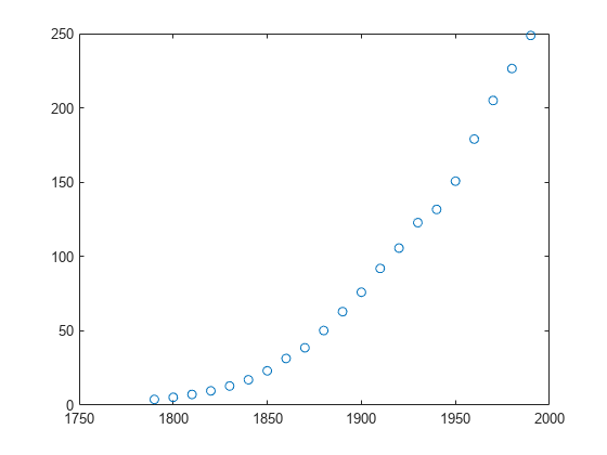

Create and Plot a Quadratic

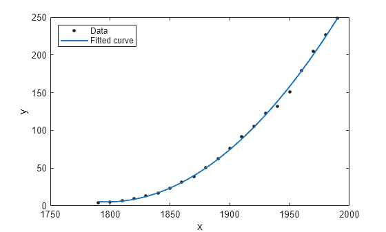
Use the fit function to fit a polynomial to data. You specify a quadratic, or second-degree polynomial, using 'poly2'. The first output from fit is the polynomial, and the second output, gof, contains the goodness of fit statistics you will examine in a later step.

[population2,gof] = fit(cdate,pop,'poly2');

To plot the fit, use the plot function. Add a legend in the top left corner.

plot(population2,cdate,pop);
legend('Location','NorthWest');

Create and Plot a Selection of Polynomials

To fit polynomials of different degrees, change the fit type, e.g., for a cubic or third-degree polynomial use 'poly3'. The scale of the input, cdate, is quite large, so you can obtain better results by centering and scaling the data. To do this, use the 'Normalize' option.

population3 = fit(cdate,pop,'poly3','Normalize','on');
population4 = fit(cdate,pop,'poly4','Normalize','on');
population5 = fit(cdate,pop,'poly5','Normalize','on');
population6 = fit(cdate,pop,'poly6','Normalize','on');

A simple model for population growth tells us that an exponential equation should fit this census data well. To fit a single term exponential model, use 'exp1' as the fittype.

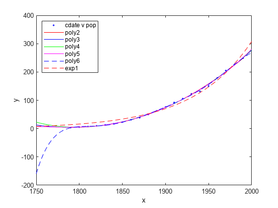
populationExp = fit(cdate,pop,'exp1');

Plot all the fits at once, and add a meaningful legend in the top left corner of the plot.

hold on
plot(population3,'b');
plot(population4,'g');
plot(population5,'m');
plot(population6,'b--');
plot(populationExp,'r--');
hold off
legend('cdate v pop','poly2','poly3','poly4','poly5','poly6','exp1', ...
    'Location','NorthWest');

Plot the Residuals to Evaluate the Fit

To plot residuals, specify 'residuals' as the plot type in the plot function.

plot(population2,cdate,pop,'residuals');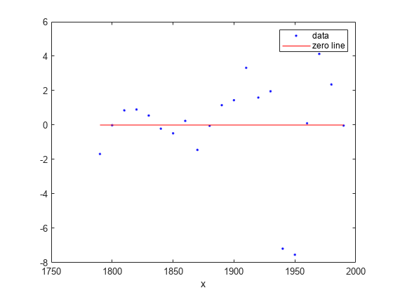

The fits and residuals for the polynomial equations are all similar, making it difficult to choose the best one.

If the residuals display a systematic pattern, it is a clear sign that the model fits the data poorly.

plot(populationExp,cdate,pop,'residuals');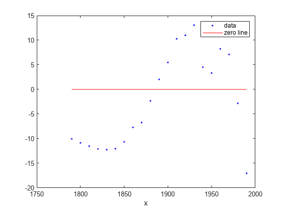

The fit and residuals for the single-term exponential equation indicate it is a poor fit overall. Therefore, it is a poor choice and you can remove the exponential fit from the candidates for best fit.

Examine Fits Beyond the Data Range

Examine the behavior of the fits up to the year 2050. The goal of fitting the census data is to extrapolate the best fit to predict future population values.

By default, the fit is plotted over the range of the data. To plot a fit over a different range, set the x-limits of the axes before plotting the fit. For example, to see values extrapolated from the fit, set the upper x-limit to 2050.

plot(cdate,pop,'o');
xlim([1900, 2050]);
hold on
plot(population6);
hold off

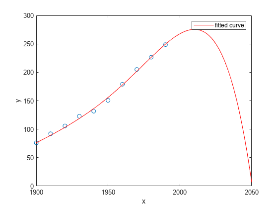
Examine the plot. The behavior of the sixth-degree polynomial fit beyond the data range makes it a poor choice for extrapolation and you can reject this fit.

Plot Prediction Intervals

To plot prediction intervals, use 'predobs' or 'predfun' as the plot type. For example, to see the prediction bounds for the fifth-degree polynomial for a new observation up to year 2050:

plot(cdate,pop,'o');
xlim([1900,2050])
hold on
plot(population5,'predobs');
hold off

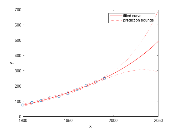
Plot prediction intervals for the cubic polynomial up to year 2050:

plot(cdate,pop,'o');
xlim([1900,2050])
hold on
plot(population3,'predobs')
hold off

Examine Goodness-of-Fit Statistics

The struct gof shows the goodness-of-fit statistics for the 'poly2' fit. When you created the 'poly2' fit with the fit function in an earlier step, you specified the gof output argument.

gof

gof = struct with fields:
           sse: 159.0293
       rsquare: 0.9987
           dfe: 18
    adjrsquare: 0.9986
          rmse: 2.9724

Examine the sum of squares due to error (SSE) and the adjusted R-square statistics to help determine the best fit. The SSE statistic is the least-squares error of the fit, with a value closer to zero indicating a better fit. The adjusted R-square statistic is generally the best indicator of the fit quality when you add additional coefficients to your model.

The large SSE for 'exp1' indicates it is a poor fit, which you already determined by examining the fit and residuals. The lowest SSE value is associated with 'poly6'. However, the behavior of this fit beyond the data range makes it a poor choice for extrapolation, so you already rejected this fit by examining the plots with new axis limits.

The next best SSE value is associated with the fifth-degree polynomial fit, 'poly5', suggesting it might be the best fit. However, the SSE and adjusted R-square values for the remaining polynomial fits are all very close to each other. Which one should you choose?

Compare the Coefficients and Confidence Bounds to Determine the Best Fit

Resolve the best fit issue by examining the coefficients and confidence bounds for the remaining fits: the fifth-degree polynomial and the quadratic.

Examine population2 and population5 by displaying the models, the fitted coefficients, and the confidence bounds for the fitted coefficients:

population2

population2 = 
     Linear model Poly2:
     population2(x) = p1*x^2 + p2*x + p3
     Coefficients (with 95% confidence bounds):
       p1 =    0.006541  (0.006124, 0.006958)
       p2 =      -23.51  (-25.09, -21.93)
       p3 =   2.113e+04  (1.964e+04, 2.262e+04)

population5

population5 = 
     Linear model Poly5:
     population5(x) = p1*x^5 + p2*x^4 + p3*x^3 + p4*x^2 + p5*x + p6
       where x is normalized by mean 1890 and std 62.05
     Coefficients (with 95% confidence bounds):
       p1 =      0.5877  (-2.305, 3.48)
       p2 =      0.7047  (-1.684, 3.094)
       p3 =     -0.9193  (-10.19, 8.356)
       p4 =       23.47  (17.42, 29.52)
       p5 =       74.97  (68.37, 81.57)
       p6 =       62.23  (59.51, 64.95)

You can also get the confidence intervals by using confint :

ci = confint(population5)

ci = 2×6

   -2.3046   -1.6841  -10.1943   17.4213   68.3655   59.5102
    3.4801    3.0936    8.3558   29.5199   81.5696   64.9469

The confidence bounds on the coefficients determine their accuracy. Check the fit equations (e.g. f(x)=p1*x+p2*x... ) to see the model terms for each coefficient. Note that p2 refers to the p2*x term in 'poly2' and the p2*x^4 term in 'poly5'. Do not compare normalized coefficients directly with non-normalized coefficients.

The bounds cross zero on the p1, p2, and p3 coefficients for the fifth-degree polynomial. This means you cannot be sure that these coefficients differ from zero. If the higher order model terms may have coefficients of zero, they are not helping with the fit, which suggests that this model over fits the census data.

The fitted coefficients associated with the constant, linear, and quadratic terms are nearly identical for each normalized polynomial equation. However, as the polynomial degree increases, the coefficient bounds associated with the higher degree terms cross zero, which suggests over fitting.

However, the small confidence bounds do not cross zero on p1, p2, and p3 for the quadratic fit, indicating that the fitted coefficients are known fairly accurately.

Therefore, after examining both the graphical and numerical fit results, you should select the quadratic population2 as the best fit to extrapolate the census data.

Evaluate the Best Fit at New Query Points

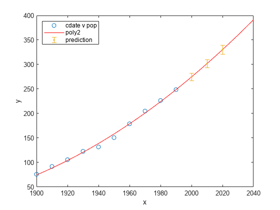
Now you have selected the best fit, population2, for extrapolating this census data, evaluate the fit for some new query points:

cdateFuture = (2000:10:2020).';
popFuture = population2(cdateFuture)

popFuture = 3×1

  274.6221
  301.8240
  330.3341

To compute 95% confidence bounds on the prediction for the population in the future, use the predint method:

ci = predint(population2,cdateFuture,0.95,'observation')

ci = 3×2

  266.9185  282.3257
  293.5673  310.0807
  321.3979  339.2702

Plot the predicted future population, with confidence intervals, against the fit and data.

plot(cdate,pop,'o');
xlim([1900,2040])
hold on
plot(population2)
h = errorbar(cdateFuture,popFuture,popFuture-ci(:,1),ci(:,2)-popFuture,'.');
hold off
legend('cdate v pop','poly2','prediction', ...
    'Location','NorthWest')

For more information, see Polynomial Models.