Plan and Execute Collision-Free Trajectories Using KINOVA Gen3 Manipulator

This example uses:

This example shows how to plan closed-loop collision-free robot trajectories from an initial to a desired end-effector pose using nonlinear model predictive control. The resulting trajectories are executed using a joint-space motion model with computed torque control. Obstacles can be static or dynamic, and can be either set as primitives (spheres, cylinders, boxes) or as custom meshes.

Robot Description and Poses

Load the KINOVA Gen3 rigid body tree (RBT) model.

robot = loadrobot('kinovaGen3', 'DataFormat', 'column');

Get the number of joints.

numJoints = numel(homeConfiguration(robot));

Specify the robot frame where the end-effector is attached.

endEffector = "EndEffector_Link";

Specify initial and desired end-effector poses. Use inverse kinematics to solve for the initial robot configuration given a desired pose.

% Initial end-effector pose
taskInit = trvec2tform([[0.4 0 0.2]])*axang2tform([0 1 0 pi]);

% Compute current robot joint configuration using inverse kinematics
ik = inverseKinematics('RigidBodyTree', robot);
ik.SolverParameters.AllowRandomRestart = false;
weights = [1 1 1 1 1 1];
currentRobotJConfig = ik(endEffector, taskInit, weights, robot.homeConfiguration);

% The IK solver respects joint limits, but for those joints with infinite
% range, they must be wrapped to a finite range on the interval [-pi, pi].
% Since the other joints are already bounded within this range, it is
% sufficient to simply call wrapToPi on the entire robot configuration
% rather than only on the joints with infinite range.
currentRobotJConfig = wrapToPi(currentRobotJConfig);

% Final (desired) end-effector pose
taskFinal = trvec2tform([0.35 0.55 0.35])*axang2tform([0 1 0 pi]);  
anglesFinal = rotm2eul(taskFinal(1:3,1:3),'XYZ');
poseFinal = [taskFinal(1:3,4);anglesFinal']; % 6x1 vector for final pose: [x, y, z, phi, theta, psi]

Collision Meshes and Obstacles

To check for and avoid collisions during control, you must setup a collision world as a set of collision objects. This example uses collisionSphere objects as obstacles to avoid. Change the following boolean to plan using static instead of moving obstacles.

isMovingObst = true;

The obstacle sizes and locations are initialized in the following helper function. To add more static obstacles, add collision objects in the world array.

helperCreateObstaclesKINOVA;

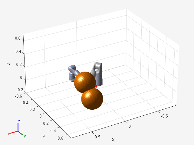
Visualize the robot at the initial configuration. You should see the obstacles in the environment as well.

x0 = [currentRobotJConfig', zeros(1,numJoints)];
helperInitialVisualizerKINOVA;

Specify a safety distance away from the obstacles. This value is used in the inequality constraint function of the nonlinear MPC controller.

safetyDistance = 0.01;

Design Nonlinear Model Predictive Controller

You can design the nonlinear model predictive controller using the following helper file, which creates an nlmpc (Model Predictive Control Toolbox) controller object. To views the file, type edit helperDesignNLMPCobjKINOVA.

helperDesignNLMPCobjKINOVA;

The controller is designed based on the following analysis. The maximum number of iterations for the optimization solver is set to 5. The lower and upper bounds for the joint position and velocities (states), and accelerations (control inputs) are set explicitly.

The robot joints model is described by double integrators. The states of the model are $x = [q, q_{}^{˙}]$ , where the 7 joint positions are denoted by $q$ and their velocities are denoted by $q_{}^{˙}$ . The inputs of the model are the joint accelerations $u = q_{}^{¨}$ . The dynamics of the model are given by

$\dot{x} = [\begin{matrix} 0 & I_{7} \\ 0 & 0 \end{matrix}] x + [\begin{matrix} 0 \\ I_{7} \end{matrix}] u$

where $I_{7}$ denotes the $7 \times 7$ identity matrix. The output of the model is defined as

$y = [\begin{matrix} I_{7} & 0 \end{matrix}] x$ .

Therefore, the nonlinear model predictive controller (nlobj) has 14 states, 7 outputs, and 7 inputs.

The cost function for nlobj is a custom nonlinear cost function, which is defined in a manner similar to a quadratic tracking cost plus a terminal cost.

$J = \int_{0}^{T} {(p_{ref} - p (q (t)))}^{'} Q_{r} (p_{ref} - p (q (t))) + u^{'} (t) Q_{u} u (t) dt + {(p_{ref} - p (q (T)))}^{'} Q_{t} (p_{ref} - p (q (T))) + {\dot{q}}^{'} (T) Q_{v} \dot{q} (T)$

Here, $p (q (t))$ transforms the joint positions $q (t)$ to the frame of end effector using forward kinematics and getTransform, and $p_{ref}$ denotes the desired end-effector pose.

The matrices $Q_{r}$ , $Q_{u}$ , $Q_{t}$ , and $Q_{v}$ are constant weight matrices.

To avoid collisions, the controller has to satisfy the following inequality constraints.

$d_{i, j} \geq d_{safe}$

Here, $d_{i, j}$ denotes the distance from the $i$ -th robot body to the $j$ -th obstacle, computed using checkCollision.

In this example, $i$ belongs to ${1, 2, 3, 4, 5, 6}$ (the base and end-effector robot bodies are excluded), and $j$ belongs to ${1, 2}$ (2 obstacles are used).

The Jacobians of the state function, output function, cost function, and inequality constraints are all provided for the prediction model to improve the simulation efficiency. To calculate the inequality constraint Jacobian, use the geometricJacobian function and the Jacobian approximation in [1].

Closed-Loop Trajectory Planning

Simulate the robot for a maximum of 50 steps with correct initial conditions.

maxIters = 50;
u0 = zeros(1,numJoints);
mv = u0;
time = 0;
goalReached = false;

Initialize the data array for control.

positions = zeros(numJoints,maxIters);
positions(:,1) = x0(1:numJoints)';

velocities = zeros(numJoints,maxIters);
velocities(:,1) = x0(numJoints+1:end)';

accelerations = zeros(numJoints,maxIters);
accelerations(:,1) = u0';

timestamp = zeros(1,maxIters);
timestamp(:,1) = time;

Use the nlmpcmove (Model Predictive Control Toolbox) function for closed-loop trajectory generation. Specify the trajectory generation options using an nlmpcmoveopt (Model Predictive Control Toolbox) object. Each iteration calculates the position, velocity, and acceleration of the joints to avoid obstacles as they move towards the goal. The helperCheckGoalReachedKINOVA script checks if the robot has reached the goal. The helperUpdateMovingObstacles script moves the obstacle locations based on the time step.

options = nlmpcmoveopt;
for timestep=1:maxIters
    disp(['Calculating control at timestep ', num2str(timestep)]);
    % Optimize next trajectory point 
    [mv,options,info] = nlmpcmove(nlobj,x0,mv,[],[], options);
    if info.ExitFlag < 0
        disp('Failed to compute a feasible trajectory. Aborting...')
        break;
    end
    % Update states and time for next iteration
    x0 = info.Xopt(2,:);
    time = time + nlobj.Ts;
    % Store trajectory points
    positions(:,timestep+1) = x0(1:numJoints)';
    velocities(:,timestep+1) = x0(numJoints+1:end)';
    accelerations(:,timestep+1) = info.MVopt(2,:)';
    timestamp(timestep+1) = time;
    % Check if goal is achieved 
    helperCheckGoalReachedKINOVA;
    if goalReached
        break;
    end
    % Update obstacle pose if it is moving
    if isMovingObst
        helperUpdateMovingObstaclesKINOVA;
    end
end

Calculating control at timestep 1

Slack variable unused or zero-weighted in your custom cost function.
All constraints will be hard.

Calculating control at timestep 2

Slack variable unused or zero-weighted in your custom cost function.
All constraints will be hard.

Calculating control at timestep 3

Slack variable unused or zero-weighted in your custom cost function.
All constraints will be hard.

Calculating control at timestep 4

Slack variable unused or zero-weighted in your custom cost function.
All constraints will be hard.

Calculating control at timestep 5

Slack variable unused or zero-weighted in your custom cost function.
All constraints will be hard.

Calculating control at timestep 6

Slack variable unused or zero-weighted in your custom cost function.
All constraints will be hard.

Calculating control at timestep 7

Slack variable unused or zero-weighted in your custom cost function.
All constraints will be hard.

Target configuration reached.

Execute Planned Trajectory using Joint-Space Robot Simulation and Control

Trim the trajectory vectors based on the time steps calculated from the plan.

tFinal = timestep+1;
positions = positions(:,1:tFinal);
velocities = velocities(:,1:tFinal);
accelerations = accelerations(:,1:tFinal);
timestamp = timestamp(:,1:tFinal);

visTimeStep = 0.2;

Use a jointSpaceMotionModel to track the trajectory with computed-torque control. The helperTimeBasedStateInputsKINOVA function generates the derivative inputs for the ode15s function for modelling the computed robot trajectory.

motionModel = jointSpaceMotionModel('RigidBodyTree',robot);

% Control robot to target trajectory points in simulation using low-fidelity model
initState = [positions(:,1);velocities(:,1)];
targetStates = [positions;velocities;accelerations]';    
[t,robotStates] = ode15s(@(t,state) helperTimeBasedStateInputsKINOVA(motionModel,timestamp,targetStates,t,state),...
                                    [timestamp(1):visTimeStep:timestamp(end)],initState);

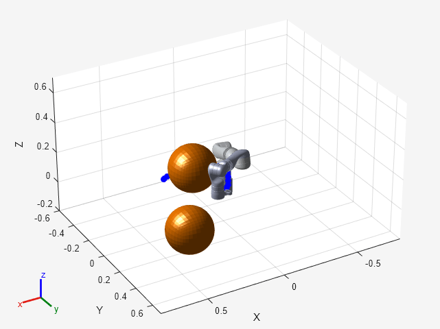
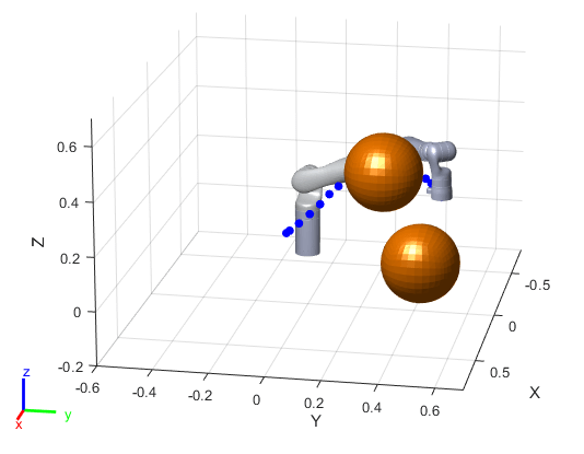
Visualize the robot motion.

helperFinalVisualizerKINOVA;

[1] Schulman, J., et al. "Motion planning with sequential convex optimization and convex collision checking." The International Journal of Robotics Research 33.9 (2014): 1251-1270.