Plan Nuclear Fuel Disposal Using Multiobjective Optimization

Model Overview

A nuclear reactor creates waste products that must be buried for long-term disposal. These waste products are fuel rod assemblies containing spent nuclear fuel. The assemblies are hot and radioactive when taken from the reactor, and gradually become less so. At period t, the radiation level is given by a double-exponential decay function with parameter vector u:

$$radiation=u_1\exp (-u_{2}t)+u_3\exp (-u_{4}t)$$.

Each assembly remains in a pool of water in the reactor building until it is cool enough to be transferred to an interim storage facility, where it is again placed in a pool of water. When the assembly is cooled further, it can be encapsulated with other assemblies in a copper-iron canister and then buried in a disposal tunnel. All disposal tunnels connect to a central tunnel.

This figure illustrates the stages of the nuclear fuel assemblies from reactor to final disposal.

The problem variables relate to a schedule where each unit of time represents 5 years. Time periods begin at 1.

Constants Associated with Model

Z is the last time period in which fuel assemblies are removed from the reactor. Removal periods are 1:Z. In [1], Z = 11. Each period is 5 years, so the last period in which fuel assemblies are removed is at time 55.

N is the last time period in which canisters are buried. Burial periods are 1:N. In [1], N = 19. Each period is 5 years, so the last period in which canisters can be buried is at time 95.

Z = 11;
N = 19;

a is the period of the last removal before the first disposal.

b is the disposal period in which the last removal occurs.

a = 5;
b = 6;

R is the minimum number of periods to store an assembly.

R = 4;

K is the maximum number of assemblies to fit into one canister.

K = 4;

T is the minimum number of canisters disposed in one period.

T = 50;

U is the maximum number of canisters disposed in one period.

U = 500;

Q is the length of a disposal tunnel in meters.

Q = 350;

M(i) is the number of assemblies removed at time i.

M = 300 - 60*(-1).^(1:Z); % 360 for odd indices, 240 for even

A(i,j) is the storage time of an assembly from removal i in period j, where i <= Z and j <= N.

A = zeros(Z,N);
for i = 1:Z
    for j = i:N
        A(i, j) = j - i;
    end
end

p(i,j) is the decay heat power of an assembly (in watts) from removal i in period j, where i <= Z and j <= N.

% The following parameters fit P_{i,j} of Table A2 from [1] to within 1 in each
% entry (fractional error <= 1/250).
u = [503 0.1346 260 0.0231];
myfun = @(d)round(u(1)*exp(-u(2)*d) + u(3)*exp(-u(4)*d));
PP = myfun(1:N);
pij = zeros(Z,N);
for i = 2:Z
    for j = 1:i
        pij(i,j) = 1e3; % Dummy values because j >= i does not occur.
    end
end
for i=1:Z
    pij(i,i:end) = PP(1:(N-i+1)); % Same decay profile for all removal times
end

pmaxup is the upper bound on the average power of a canister, and pmaxlow is the lower bound.

pmaxup = 1830;
pmaxlow = 1300;

dDTup is the upper bound on the distance between disposal tunnels, and dDTlow is the lower bound.

dDTup = 50;
dDTlow = 25;

dCAup is the upper bound on the distance between canisters in a disposal tunnel, and dCAlow is the lower bound.

dCAup = 15;
dCAlow = 6;

The costs associated with the operations are not given in [1]. This example assumes the following values:

Cas = 50;
Cis = 60;
Csp = 10;
Cca = 1200;
Cef = 300;
Cdt = 3000;
Cct = 5000;

Optimization Variables for Problem

To create the problem for MATLAB®, use the problem-based approach. Define continuous variables for most quantities.

This figure illustrates the variables associated with the movement of the assemblies.

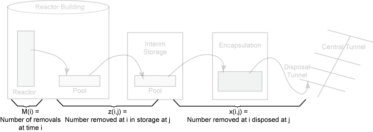
x(i,j) is the number of assemblies removed at time i and disposed at time j, i <= Z and j <= N.

x = optimvar("x",Z,N,LowerBound=0,UpperBound=U*K);

z(i,j) is the number of assemblies removed at time i and in storage at time j, i <= Z and j <= N.

z = optimvar("z",Z,N,LowerBound=0,UpperBound=U*K*N/2);

y(j) is the number of canisters disposed at time j <= N.

y = optimvar("y",N,LowerBound=0,UpperBound=U);

pmax is the maximum average power of a canister.

pmax = optimvar("pmax",LowerBound=pmaxlow,UpperBound=pmaxup);

This figure illustrates quantities associated with the disposal tunnels.

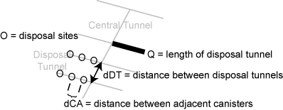
dDT is the distance between adjacent disposal tunnels.

dDT = optimvar("dDT",LowerBound=dDTlow,UpperBound=dDTup);

dCA is the distance between adjacent canisters in a disposal tunnel. You compute this distance later on, in the Problem Constraints section of this example, using the function g.

This figure relates to the encapsulation times.

Specify the following variables as integer type binary variables, which have lower bounds of 0 and upper bounds of 1.

ej(j) indicates that the encapsulation facility is in operation during the period j <= N.

ej = optimvar("ej",N,Type="integer",LowerBound=0,UpperBound=1);

ejON(j) indicates that encapsulation starts at the beginning of period j <= N.

ejON = optimvar("ejON",N,Type="integer",LowerBound=0,UpperBound=1);

ejOFF(j) indicates that encapsulation ends at the beginning of period j <= N.

ejOFF = optimvar("ejOFF",N,Type="integer",LowerBound=0,UpperBound=1);

This figure relates to the times when assemblies can be disposed, rij = 1. These times start when ejON = 1 and end when sij = 1.

sij(i,j) indicates that assemblies removed at time i can no longer be disposed starting at the beginning of time j, i <= Z and j <= N.

sij = optimvar("sij",Z,N,Type="integer",LowerBound=0,UpperBound=1);

rij(i,j) indicates that assemblies removed at time i can be disposed at time j, i <= Z and j <= N.

rij = optimvar("rij",Z,N,Type="integer",LowerBound=0,UpperBound=1);

All optimization variables and problem parameters are now defined.

Problem Constraints

Create an optimization problem to hold the objective and constraints.

prob = optimproblem;

The constraint numbers match the equations in [1]. The first three constraints relate to the number of assemblies in interim storage.

jnot1 = 2:N;
prob.Constraints.cons10 = z(:,1) - M(:) + x(:,1) == 0;
prob.Constraints.cons11 = z(:,jnot1) - z(:,(jnot1 - 1)) + x(:,jnot1) == 0;
prob.Constraints.cons12 = z(:,N) == 0;

Set the constraint that all assemblies are disposed once.

prob.Constraints.cons13 = sum(sij,2) == 1;

Define the variable rij by setting the following constraints.

cons15 = optimconstr(Z,N);
cons15(:,1) = rij(:,1) == -sij(:,1) + ejON(1); % equation 14
cons15(:,jnot1) = rij(:,jnot1) == ...
    rij(:,jnot1-1) - sij(:,jnot1) + repmat(ejON(jnot1)',Z,1); % equation 15
prob.Constraints.cons15 = cons15;

Set the constraint that disposal occurs only during times when the encapsulation facility is in operation.

cons16 = rij <= repmat(ej', Z, 1);
prob.Constraints.cons16 = cons16;

Specify the constraint that production capacity is not exceeded.

prob.Constraints.cons17 = x <= U*K*rij;

The next constraint enforces that assemblies are cool enough before disposal.

prob.Constraints.cons18 = x.*(A - R) >= 0;

The following constraints relate to the encapsulation facility. These constraints enforce that the facility is turned on and off only once, which means that all canisters are encapsulated in one run,

prob.Constraints.cons19 = sum(ejON) == 1;
prob.Constraints.cons20 = sum(ejOFF) == 1;

Define variable ej by setting the following constraints.

cons21 = optimconstr(N);
cons21(1) = ej(1) == ejON(1) - ejOFF(1); % equation 21
cons21(jnot1) = ej(jnot1) == ...
    ej(jnot1 - 1) + ejON(jnot1) - ejOFF(jnot1); % equation 22
prob.Constraints.cons21 = cons21;

Set constraints that the number of canisters is sufficient for disposal, does not exceed production capacity, and obeys the minimum production constraint.

prob.Constraints.cons23 = y' >= (1/K)*sum(x,1);
prob.Constraints.cons24 = y <= U*ej;
jnotN = 1:(N-1);
prob.Constraints.cons25 = y(jnotN) >= T*(ej(jnotN) - ejOFF(jnotN + 1));

Regarding the disposal facility, set the constraint that the heat power of canisters is allowable.

prob.Constraints.cons26 = sum(pij.*x,1) <= pmax*y';

Specify a nonlinear constraint on the distance between buried canisters. The function is piecewise linear, and is defined using the max function, which is not a supported operation for optimization expressions. Therefore, use fcn2optimexpr to place the constraint into prob.

g = @(pmax,dDT)max([-2.26911*dDT + 0.00675*pmax + 54.5288,...
    -0.05833*dDT + 0.00596*pmax - 0.727083,...
    -0.14*dDT + 0.17701*pmax - 350.651]);
dCA = fcn2optimexpr(@(pmax,dDT)g(pmax,dDT),pmax,dDT);
prob.Constraints.cons29a = dCA >= dCAlow;
prob.Constraints.cons29b = dCA <= dCAup;

Cost Objective

The first objective for this multiobjective problem is the cost, which has seven components.

cost = optimexpr(7,1);

1. Storage cost of assemblies. This cost is the sum of the cost per unit time multiplied by the length of time each assembly is stored.

cost(1) = Cas*sum(A.*x,"all");

2. Cost of interim storage. This cost is j*ejOFF(j) for the one component of ejOFF that is 1.

cost(2) = Cis*max(ejOFF(1)–1,2*ejOFF(2)–1,3*ejOFF(3)–1,...,N*ejOFF(N)–1).

To represent this expression briefly, represent cost(2) = Cis*u for a new optimization variable u, along with the constraint

ucons = u >= ((1:N)'.*ejOFF) – 1.

u = optimvar("u",LowerBound=0);
cost(2) = Cis*u;
ucons = u >= ((1:N)'.*ejOFF) - 1;
prob.Constraints.ucons = ucons;

3. Cost of positions for assembly storage. cost(3) can be represented by Csp*v1, where v1 is a new optimization variable, along with the constraints

v1 >= sum(M)

v1 >= sum_{i=1}^j z(i,j) for each 1 <= j <= N

v1 >= sum_{i=1}^Z z(i,j) for each b <= j <= N.

Create these costs and associated constraints.

v1 = optimvar("v1",LowerBound=0);
cost(3) = Csp*v1; % Include the three v1 constraints given below.
v1consa = v1 >= sum(M);
bmin1 = 1:(b-1);
v1consb = optimconstr(b-1);
for j=bmin1
    v1consb(j) = sum(z(1:a+j,j)) <= v1;
end
ell = b:N;
v1consc = sum(z(:,ell),1) <= v1;
prob.Constraints.v1consa = v1consa;
prob.Constraints.v1consb = v1consb;
prob.Constraints.v1consc = v1consc;

4. Cost of canisters. This cost is the cost per canister times the total number of canisters buried.

cost(4) = Cca*sum(y);

5. Cost of running the encapsulation facility. This cost is the cost per unit time multiplied by the length of time the facility operates.

cost(5) = Cef*sum(ej);

6. Cost of disposal tunnels. This is the cost per unit length times the length between canisters times the total number of canisters buried.

cost(6) = Cdt*dCA*sum(y);

7. Cost of central tunnel. This cost is the cost per unit length times the required length of the central tunnel. The number of canisters that can be buried in one disposal tunnel is its length Q divided by the distance between canisters dCA. The length of the central tunnel is proportional to the number of buried canisters sum(y) and inversely proportional to Q/dCA, and has cost proportional to Cct.

cost(7) = Cct/Q*dDT*dCA*sum(y);

The total cost is the sum of the seven cost components. To change the scale of the total cost to match that of the other objectives, take the logarithm of the sum.

prob.Objective.cost = log(sum(cost));

Safety Objectives

The problem has two objectives related to safety. Objective 2, named safety1, tries to minimize the maximum storage time over all removals. Objective 3, named safety2, tries to stop the disposal as early as possible. Define these two objectives using the helper functions max1 and max2, which appear at the end of this script.

prob.Objective.safety1 = fcn2optimexpr(@max1,A,sij);
% Minimize maximum storage time, objective (2) in [1]

prob.Objective.safety2 = fcn2optimexpr(@max2,ejOFF);
% Stop disposal as early as possible, objective (5) in [1]

Set Options

Set the options for a Pareto plot as the solver proceeds. Because the problem has over 900 variables, set options to use a population size of 500, which is larger than the default. Also, because the problem contains binary variables, use the mutationgaussian mutation function. This mutation function works better than the default mutationpower for binary variables.

opts = optimoptions("gamultiobj",PlotFcn="gaplotpareto",PopulationSize=5e2,...
    MutationFcn=@mutationgaussian);

Run Problem

The problem formulation is complete, and the options are set for this multiobjective problem. Run the problem.

rng default % For reproducibility
[sol,fval,exitflag,output] = solve(prob,Options=opts);

Solving problem using gamultiobj.
gamultiobj stopped because the average change in the spread of Pareto solutions is less than options.FunctionTolerance.

xlabel("Cost")
ylabel("Safety 1")
zlabel("Safety 2")

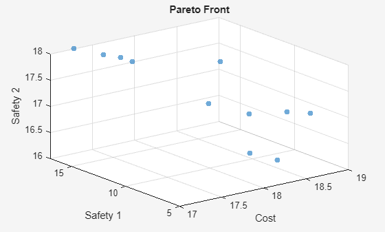
The Pareto plot shows a clear tradeoff between Cost and Safety 1. The true cost is the exponential of the amount shown, so the tradeoff is more severe than illustrated.

Examine Solution

gamultiobj finds several feasible solutions with varying fitness function values. To find the control variables associated with the solutions, use the data tips.

After activating Data Tips, click the upper-left solution.

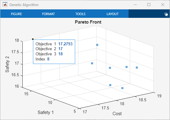
The index of the selected point is 4. The variables associated with this point are in sol(4).

Examine the x variables associated with this solution. Recall that x(i,j) are the removals at time i that are disposed at time j.

disp(sol(4).x)

         0         0         0         0         0         0         0         0         0         0         0         0         0         0         0         0  360.0000         0         0
         0         0         0         0         0         0         0         0         0         0         0         0         0         0         0         0  240.0000         0         0
         0         0         0         0         0         0         0         0         0         0         0         0         0         0         0         0  265.4535   94.5465         0
         0         0         0         0         0         0         0         0         0         0         0         0         0         0         0         0  240.0000         0         0
         0         0         0         0         0         0         0         0         0         0         0         0         0         0         0         0         0  360.0000         0
         0         0         0         0         0         0         0         0         0         0         0         0         0         0         0         0         0  240.0000         0
         0         0         0         0         0         0         0         0         0         0         0         0         0         0         0         0  254.5465  105.4535         0
         0         0         0         0         0         0         0         0         0         0         0         0         0         0         0         0         0  240.0000         0
         0         0         0         0         0         0         0         0         0         0         0         0         0         0         0         0         0  360.0000         0
         0         0         0         0         0         0         0         0         0         0         0         0         0         0         0         0         0  240.0000         0
         0         0         0         0         0         0         0         0         0         0         0         0         0         0         0         0         0  360.0000         0

Clearly, the x schedule is not restricted to integer values. View the sums of the x schedule over disposals compared to the removal quantities M(:).

disp([sum(sol(4).x,2),M(:)])

   360   360
   240   240
   360   360
   240   240
   360   360
   240   240
   360   360
   240   240
   360   360
   240   240
   360   360

The x schedule accounts for all removals.

What are the times when the encapsulation facility is in operation?

disp(sol(4).ej')

     0     0     0     0     0     0     0     0     0     0     0     0     0     0     0     0     1     1     0

The encapsulation runs for times 17 and 18.

What is the distance between disposal tunnels?

disp(sol(4).dDT)

   27.6483

The distance is greater than but close to its lower bound of 25.

What is the dollar cost of the schedule? To find out, calculate exp(sol(4).cost), because sol(4).cost is the logarithm of the total disposal cost.

disp(exp(sol(4).cost))

   2.0883e+07

The cost is about $21 million.

Examine the point in the Pareto set with the lowest value of Objective 2.

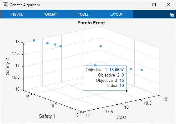
The index of this point is 3. The monetary cost of this operating point is much higher.

disp(exp(sol(3).cost))

   1.4001e+08

The monetary cost is about $140 million, which is over six times the previous value. But the gain is that Objective 2 is 10 instead of 17, which corresponds to waste burial that is 35 (=7*5) years earlier. Earlier burial can be considered safer.

View the schedule of x for this solution.

disp(sol(3).x)

     0     0     0     0     0     0     0     0   360     0     0     0     0     0     0     0     0     0     0
     0     0     0     0     0   240     0     0     0     0     0     0     0     0     0     0     0     0     0
     0     0     0     0     0     0     0     0     0   160     0   200     0     0     0     0     0     0     0
     0     0     0     0     0     0     0     0     0     0   240     0     0     0     0     0     0     0     0
     0     0     0     0     0     0     0     0   360     0     0     0     0     0     0     0     0     0     0
     0     0     0     0     0     0     0     0     0     0   240     0     0     0     0     0     0     0     0
     0     0     0     0     0     0     0     0     0     0   360     0     0     0     0     0     0     0     0
     0     0     0     0     0     0     0     0     0     0     0     0     0     0   240     0     0     0     0
     0     0     0     0     0     0     0     0     0     0     0     0     0   360     0     0     0     0     0
     0     0     0     0     0     0     0     0     0     0     0     0     0     0     0     0     0   240     0
     0     0     0     0     0     0     0     0     0     0     0     0     0     0   360     0     0     0     0

View the sums of the x schedule over disposals compared to the removal quantities M(:).

disp([sum(sol(3).x,2),M(:)])

   360   360
   240   240
   360   360
   240   240
   360   360
   240   240
   360   360
   240   240
   360   360
   240   240
   360   360

Again, the schedule accounts for all removals.

What are the times when the encapsulation facility is in operation?

disp(sol(3).ej')

     1     1     1     1     1     1     1     1     1     1     1     1     1     1     1     1     1     1     0

The encapsulation runs for times 1 through 18.

What is the distance between disposal tunnels for this solution?

disp(sol(3).dDT)

   38.4942

This time, the distance between disposal tunnels is about halfway between the lower bound of 25 meters and upper bound of 50 meters.

Conclusion

This example shows the formulation of a nonlinear, multiobjective, mixed-integer optimization problem using the problem-based approach. The Data Tips in the Pareto plot enable you to analyze the solution. Instead of specifying the gaplotpareto plot function, you can use the paretoplot function to obtain a similar plot from the solution.

References

[1] Montonen, Outi, Timo Ranta, and Marko M. Mäkelä. Planning the Schedule for the Disposal of the Spent Nuclear Fuel with Interactive Multiobjective Optimization. Algorithms Vol. 12, Issue 12, 2019. Available at https://www.mdpi.com/1999-4893/12/12/252.

Helper Functions

This code creates the max1 helper function.

function v = max1(A,sij)
v = round(max(max(A.*sij - 1))); % "round" ensures integer values
end

This code creates the max2 helper function.

function v = max2(ejOFF)
v = round(max((ejOFF').*(1:length(ejOFF)) - 1));
end