Fit ODE Parameters Using Optimization Variables

Problem

The problem is a multistep reaction model involving several substances, some of which react with each other to produce different substances.

For this problem, the true reaction rates are unknown. So, you need to observe the reactions and infer the rates. Assume that you can measure the substances for a set of times $$t$$. From these observations, fit the best set of reaction rates to the measurements.

Model

The model has six substances, $$C_1$$ through $$C_6$$, that react as follows:

The reaction rate is proportional to the product of the quantities of the required substances. So, if $$y_i$$ represents the quantity of substance $$C_i$$, then the reaction rate to produce $$C_3$$ is $$r_1{y}_1{y}_2$$. Similarly, the reaction rate to produce $$C_5$$ is $$r_2{y}_3{y}_4$$, and the reaction rate to produce $$C_6$$ is $$r_3{y}_3{y}_4$$.

In other words, the differential equation controlling the evolution of the system is

Start the differential equation at time 0 at the point $$y(0)=[1,1,0,1,0,0]$$. These initial values ensure that all of the substances react completely, causing $$C_1$$ through $$C_4$$ to approach zero as time increases.

Express Model in MATLAB

The diffun function implements the differential equations in a form ready for solution by ode45.

type diffun

function dydt = diffun(~,y,r)
dydt = zeros(6,1);
s12 = y(1)*y(2);
s34 = y(3)*y(4);

dydt(1) = -r(1)*s12;
dydt(2) = -r(1)*s12;
dydt(3) = -r(2)*s34 + r(1)*s12 - r(3)*s34;
dydt(4) = -r(2)*s34 - r(3)*s34;
dydt(5) = r(2)*s34;
dydt(6) = r(3)*s34;
end

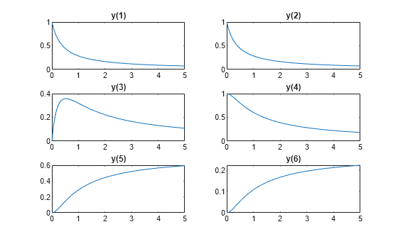
The true reaction rates are $$r_1=2.5$$, $$r_2=1.2$$, and $$r_3=0.45$$. Compute the evolution of the system for times zero through five by calling ode45.

rtrue = [2.5 1.2 0.45];
y0 = [1 1 0 1 0 0];
tspan = linspace(0,5);
soltrue = ode45(@(t,y)diffun(t,y,rtrue),tspan,y0);
yvalstrue = deval(soltrue,tspan);
for i = 1:6
    subplot(3,2,i)
    plot(tspan,yvalstrue(i,:))
    title(['y(',num2str(i),')'])
end

Optimization Problem

To prepare the problem for solution in the problem-based approach, create a three-element optimization variable r that has a lower bound of 0.1 and an upper bound of 10.

r = optimvar('r',3,"LowerBound",0.1,"UpperBound",10);

The objective function for this problem is the sum of squares of the differences between the ODE solution with parameters r and the solution with the true parameters yvals. To express this objective function, first write a MATLAB function that computes the ODE solution using parameters r. This function is the RtoODE function.

type RtoODE

function solpts = RtoODE(r,tspan,y0)
sol = ode45(@(t,y)diffun(t,y,r),tspan,y0);
solpts = deval(sol,tspan);
end

To use RtoODE in an objective function, convert the function to an optimization expression by using fcn2optimexpr. See Convert Nonlinear Function to Optimization Expression.

myfcn = fcn2optimexpr(@RtoODE,r,tspan,y0);

Express the objective function as the sum of squared differences between the ODE solution and the solution with true parameters.

obj = sum(sum((myfcn - yvalstrue).^2));

Create an optimization problem with the objective function obj.

prob = optimproblem("Objective",obj);

Solve Problem

To find the best-fitting parameters r, give an initial guess r0 for the solver and call solve.

r0.r = [1 1 1];
[rsol,sumsq] = solve(prob,r0)

Solving problem using lsqnonlin.

Local minimum found.

Optimization completed because the size of the gradient is less than
the value of the optimality tolerance.

rsol = struct with fields:
    r: [3x1 double]

sumsq = 3.8661e-15

The sum of squared differences is essentially zero, meaning the solver found parameters that cause the ODE solution to match the solution with true parameters. So, as expected, the solution contains the true parameters.

disp(rsol.r)

    2.5000
    1.2000
    0.4500

disp(rtrue)

    2.5000    1.2000    0.4500

Limited Observations

Suppose that you cannot observe all the components of y, but only the final outputs y(5) and y(6). Can you obtain the values of all the reaction rates based on this limited information?

To find out, modify the function RtoODE to return only the fifth and sixth ODE outputs. The modified ODE solver is in RtoODE2.

type RtoODE2

function solpts = RtoODE2(r,tspan,y0)
solpts = RtoODE(r,tspan,y0);
solpts = solpts([5,6],:); % Just y(5) and y(6)
end

The RtoODE2 function simply calls RtoODE and then takes the final two rows of the output.

Create a new optimization expression from RtoODE2 and the optimization variable r, the time span data tspan, and the initial point y0.

myfcn2 = fcn2optimexpr(@RtoODE2,r,tspan,y0);

Modify the comparison data to include outputs 5 and 6 only.

yvals2 = yvalstrue([5,6],:);

Create a new objective and new optimization problem from the optimization expression myfcn2 and the comparison data yvals2.

obj2 = sum(sum((myfcn2 - yvals2).^2));
prob2 = optimproblem("Objective",obj2);

Solve the problem based on this limited set of observations.

[rsol2,sumsq2] = solve(prob2,r0)

Solving problem using lsqnonlin.

Local minimum possible.

lsqnonlin stopped because the final change in the sum of squares relative to 
its initial value is less than the value of the function tolerance.

rsol2 = struct with fields:
    r: [3x1 double]

sumsq2 = 2.1616e-05

Once again, the returned sum of squares is essentially zero. Does this mean that the solver found the correct reaction rates?

disp(rsol2.r)

    1.7811
    1.5730
    0.5899

disp(rtrue)

    2.5000    1.2000    0.4500

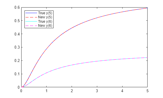
No; in this case, the new rates are quite different from the true rates. However, a plot of the new ODE solution compared to the true values shows that y(5) and y(6) match the true values.

figure
plot(tspan,yvals2(1,:),'b-')
hold on
ss2 = RtoODE2(rsol2.r,tspan,y0);
plot(tspan,ss2(1,:),'r--')
plot(tspan,yvals2(2,:),'c-')
plot(tspan,ss2(2,:),'m--')
legend('True y(5)','New y(5)','True y(6)','New y(6)','Location','northwest')
hold off

To identify the correct reaction rates for this problem, you must have data for more observations than y(5) and y(6).

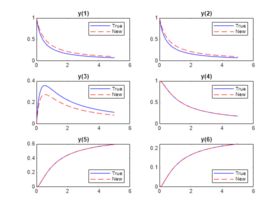
Plot all the components of the solution with the new parameters, and plot the solution with the true parameters.

figure
yvals2 = RtoODE(rsol2.r,tspan,y0);
for i = 1:6
    subplot(3,2,i)
    plot(tspan,yvalstrue(i,:),'b-',tspan,yvals2(i,:),'r--')
    legend('True','New','Location','best')
    title(['y(',num2str(i),')'])
end

With the new parameters, substances $$C_1$$ and $$C_2$$ drain more slowly, and substance $$C_3$$ does not accumulate as much. But substances $$C_4$$, $$C_5$$, and $$C_6$$ have exactly the same evolution with both the new parameters and the true parameters.