Evaluate Curve Fit

This example shows how to work with a curve fit.

Load Data and Fit a Polynomial Curve

load census
curvefit = fit(cdate,pop,'poly3','normalize','on')

curvefit = 
     Linear model Poly3:
     curvefit(x) = p1*x^3 + p2*x^2 + p3*x + p4
       where x is normalized by mean 1890 and std 62.05
     Coefficients (with 95% confidence bounds):
       p1 =       0.921  (-0.9743, 2.816)
       p2 =       25.18  (23.57, 26.79)
       p3 =       73.86  (70.33, 77.39)
       p4 =       61.74  (59.69, 63.8)

The output displays the fitted model equation, the fitted coefficients, and the confidence bounds for the fitted coefficients.

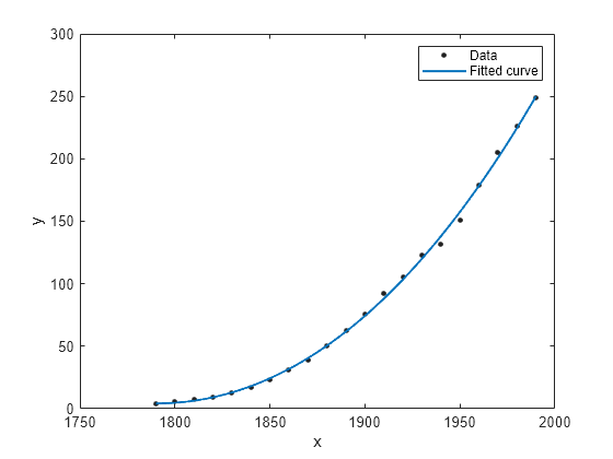
Plot the Fit, Data, Residuals, and Prediction Bounds

plot(curvefit,cdate,pop)

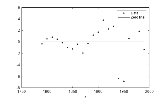
Plot the residuals fit.

plot(curvefit,cdate,pop,'Residuals')

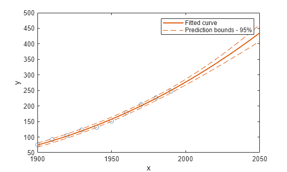
Plot the prediction bounds on the fit.

plot(curvefit,cdate,pop,'predfunc')

Evaluate the Fit at a Specified Point

Evaluate the fit at a specific point by specifying a value for x , using this form: y = fittedmodel(x).

curvefit(1991)

ans = 252.6690

Evaluate the Fit Values at Many Points

Evaluate the model at a vector of values to extrapolate to the year 2050.

xi = (2000:10:2050).';
curvefit(xi)

Get prediction bounds on those values.

ci = predint(curvefit,xi)

ci = 6×2

  267.8589  286.0674
  294.3070  316.5770
  321.5924  349.4208
  349.7275  384.6329
  378.7255  422.2462
  408.5919  462.3017

Plot the fit and prediction intervals across the extrapolated fit range. By default, the fit is plotted over the range of the data. To see values extrapolated from the fit, set the upper x-limit of the axes to 2050 before plotting the fit. To plot prediction intervals, use predobs or predfun as the plot type.

plot(cdate,pop,'o')
xlim([1900,2050])
hold on
plot(curvefit,'predobs')
hold off

Get the Model Equation

Enter the fit name to display the model equation, the fitted coefficients, and the confidence bounds for the fitted coefficients.

curvefit

curvefit = 
     Linear model Poly3:
     curvefit(x) = p1*x^3 + p2*x^2 + p3*x + p4
       where x is normalized by mean 1890 and std 62.05
     Coefficients (with 95% confidence bounds):
       p1 =       0.921  (-0.9743, 2.816)
       p2 =       25.18  (23.57, 26.79)
       p3 =       73.86  (70.33, 77.39)
       p4 =       61.74  (59.69, 63.8)

To get only the model equation, use formula.

formula(curvefit)

ans = 
'p1*x^3 + p2*x^2 + p3*x + p4'

Get Coefficient Names and Values

Specify a coefficient by name.

p1 = curvefit.p1

p1 = 0.9210

p2 = curvefit.p2

p2 = 25.1834

Get all the coefficient names. Look at the fit equation (for example, f(x) = p1*x^3+... ) to see the model terms for each coefficient.

coeffnames(curvefit)

ans = 4x1 cell
    {'p1'}
    {'p2'}
    {'p3'}
    {'p4'}

Get all the coefficient values.

coeffvalues(curvefit)

ans = 1×4

    0.9210   25.1834   73.8598   61.7444

Get Confidence Bounds on the Coefficients

Use confidence bounds on coefficients to help you evaluate and compare fits. The confidence bounds on the coefficients determine their accuracy. Bounds that are far apart indicate uncertainty. If the bounds cross zero for linear coefficients, this means you cannot be sure that these coefficients differ from zero. If some model terms have coefficients of zero, then they are not helping with the fit.

confint(curvefit)

ans = 2×4

   -0.9743   23.5736   70.3308   59.6907
    2.8163   26.7931   77.3888   63.7981

Examine Goodness-of-Fit Statistics

To get goodness-of-fit statistics at the command line, you can either:

Open the Curve Fitter app. On the Curve Fitter tab, in the Export section, click Export and select Export to Workspace to export your fit and goodness of fit to the workspace.
Specify the gof output argument using the fit function.

Recreate the fit specifying the gof and output arguments to get goodness-of-fit statistics and fitting algorithm information.

[curvefit,gof,output] = fit(cdate,pop,'poly3','normalize','on')

curvefit = 
     Linear model Poly3:
     curvefit(x) = p1*x^3 + p2*x^2 + p3*x + p4
       where x is normalized by mean 1890 and std 62.05
     Coefficients (with 95% confidence bounds):
       p1 =       0.921  (-0.9743, 2.816)
       p2 =       25.18  (23.57, 26.79)
       p3 =       73.86  (70.33, 77.39)
       p4 =       61.74  (59.69, 63.8)

gof = struct with fields:
           sse: 149.7687
       rsquare: 0.9988
           dfe: 17
    adjrsquare: 0.9986
          rmse: 2.9682

output = struct with fields:
        numobs: 21
      numparam: 4
     residuals: [21x1 double]
      Jacobian: [21x4 double]
      exitflag: 1
     algorithm: 'QR factorization and solve'
    iterations: 1

Plot a histogram of the residuals to look for a roughly normal distribution.

histogram(output.residuals,10)

Plot the Fit, Data, and Residuals

plot(curvefit,cdate,pop,'fit','residuals')
legend Location SouthWest
subplot(2,1,1)
legend Location NorthWest

Find Methods

List every method that you can use with the fit.

methods(curvefit)

Methods for class cfit:

argnames       category       cfit           coeffnames     coeffvalues    confint        dependnames    differentiate  feval          fitoptions     formula        indepnames     integrate      islinear       numargs        numcoeffs      plot           predint        probnames      probvalues     setoptions     type

For more information on how to use a fit method, see cfit.