Custom Linear Fitting

About Custom Linear Models

In the Curve Fitter app, you can use the Custom Equation fit to define your own linear or nonlinear equations. The custom equation fit uses the nonlinear least-squares fitting procedure.

You can define a custom linear equation in Custom Equation, but the nonlinear fitting is less efficient and usually slower than linear least-squares fitting. If you need linear least-squares fitting for custom equations, select Linear Fitting instead. Linear models are linear combinations of (perhaps nonlinear) terms. They are defined by equations that are linear in the parameters.

Tip

If you need linear least-squares fitting for custom equations, choose Linear Fitting. If you don’t know if your equation can be expressed as a set of linear functions, then choose Custom Equation instead. See Selecting a Custom Equation Fit Interactively.

Selecting a Linear Fitting Custom Fit Interactively

In the Curve Fitter app, select some curve data. On the Curve Fitter tab, in the Data section, click Select Data. In the Select Fitting Data dialog box, select X data and Y data values.
Curve Fitter creates a default polynomial fit.
Change the model type. On the Curve Fitter tab, in the Fit Type section, click the arrow to open the gallery. In the gallery, click Linear Fitting in the Custom group.
In the Fit Options pane, an example equation appears when you click Linear Fitting.
You can change x and y to any valid variable names.
The lower box displays the example equation. Change the Coefficients and Terms entries to change the example terms and define your own equation.

For an example, see Fit Custom Linear Legendre Polynomials in Curve Fitter App.

Selecting Linear Fitting at the Command Line

To use a linear fitting algorithm, specify a cell array or string array of model terms as an input to the fit or fittype functions. Do not include coefficients in the expressions for the terms. If there is a constant term, use '1' as the corresponding expression in the array.

To specify a linear model of the following form:

 coeff1 * term1 + coeff2 * term2 + coeff3 * term3 + ...

where no coefficient appears within any of term1, term2, etc., use a cell array or string array where each term, without coefficients, is specified as a separate element. For example:

LinearModelTerms = {'term1', 'term2', 'term3', ... }

Identify the linear model terms you need to input to fittype. For example, the model
```
a*log(x) + b*x + c
```
is linear in a, b, and c. It has three terms log(x), x, and 1 (because c=c*1). To specify this model you use these terms: LinearModelTerms = {'log(x)','x','1'}.

Use the cell array or string array of linear model terms as the input to the fittype function:

linearfittype = fittype({'log(x)','x','1'})

linearfittype = 

     Linear model:
     linearfittype(a,b,c,x) = a*log(x) + b*x + c

Load some data and use the fittype as an input to the fit function.

load census
f = fit(cdate,pop,linearfittype)

f = 

     Linear model:
     f(x) = a*log(x) + b*x + c
     Coefficients (with 95% confidence bounds):
       a =  -4.663e+04  (-4.973e+04, -4.352e+04)
       b =        25.9  (24.26, 27.55)
       c =   3.029e+05  (2.826e+05, 3.232e+05)

Alternatively, you can specify the cell array or string array of linear model terms as an input to the fit function:

f = fit(x,z,{'log(x)','x','1'})

Plot the fit and data.
```
plot(f,cdate,pop)
```

For an example, see Fit Custom Linear Legendre Polynomials at the Command Line.

Fit Custom Linear Legendre Polynomials

Fit Custom Linear Legendre Polynomials in Curve Fitter App

This example shows how to fit data using several custom linear equations. The data is generated, and is based on the nuclear reaction ¹²C(e,e'α)⁸Be. The equations use sums of Legendre polynomial terms.

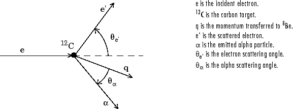
Consider an experiment in which 124 MeV electrons are scattered from ¹²C nuclei. In the subsequent reaction, alpha particles are emitted and produce the residual nuclei ⁸Be. By analyzing the number of alpha particles emitted as a function of angle, you can deduce certain information regarding the nuclear dynamics of ¹²C. The reaction kinematics are shown next.

The data is collected by placing solid state detectors at values of Θ_α ranging from 10^o to 240^o in 10^o increments.

It is sometimes useful to describe a variable expressed as a function of angle in terms of Legendre polynomials

$y (x) = \sum_{n = 0}^{\infty} a_{n} P_{n} (x)$

where P_n(x) is a Legendre polynomial of degree n, x is cos(Θ_α), and a_n are the coefficients of the fit. For information about generating Legendre polynomials, see the legendre function.

For the alpha-emission data, you can directly associate the coefficients with the nuclear dynamics by invoking a theoretical model. Additionally, the theoretical model introduces constraints for the infinite sum shown above. In particular, by considering the angular momentum of the reaction, a fourth-degree Legendre polynomial using only even terms should describe the data effectively.

You can generate Legendre polynomials with Rodrigues' formula:

$P_{n} (x) = \frac{1}{2^{n} n!} {(\frac{d}{d x})}^{n} {(x^{2} - 1)}^{n}$

Legendre Polynomials Up to Fourth Degree

n	P_n(x)
0	1
1	x
2	(1/2)(3x²– 1)
3	(1/2)(5x³ – 3x)
4	(1/8)(35x⁴ – 30x² + 3)

This example shows how to fit the data using a fourth-degree Legendre polynomial with only even terms:

$y_{1} (x) = a_{0} + a_{2} (\frac{1}{2}) (3 x^{2} - 1) + a_{4} (\frac{1}{8}) (35 x^{4} - 30 x^{2} + 3)$

Load the ¹²C alpha-emission data.
```
load carbon12alpha
```
The workspace now contains two new variables:
- angle is a vector of angles (in radians) ranging from 10^o to 240^o in 10^o increments.
- counts is a vector of raw alpha particle counts that correspond to the emission angles in angle.
Open the Curve Fitter app.
```
curveFitter
```
In the Curve Fitter app, on the Curve Fitter tab, in the Data section, click Select Data. In the Select Fitting Data dialog box, select angle and counts as the X data and Y data values, respectively, to create a default polynomial fit to the two variables.
Change the fit type to a default custom linear fit. On the Curve Fitter tab, in the Fit Type section, click the arrow to open the gallery. In the gallery, click Linear Fitting in the Custom group.
Use Linear Fitting instead of the Custom Equation fit type because the Legendre polynomials depend only on the predictor variable and constants. The equation you will specify for the model is y₁(x) (that is, the equation given at the beginning of this procedure). Because angle is given in radians, the argument of the Legendre terms is given by cos(Θ_α).
In the Fit Options pane, change the equation terms.
1. Change the Coefficients names to a2, a4, and a0.
2. Change the Terms value for a2 to the following:
  (1/2)*(3*cos(x)^2-1)
  The Curve Fitter app updates the fit as you edit the terms.
3. Change the Terms value for a4 to the following:
  (1/8)*(35*cos(x)^4-30*cos(x)^2+3)
  The fit appears in the Curve Fitter app.
In the Table Of Fits pane, double-click the Fit name value and change it to Leg4Even.
Display the residuals. On the Curve Fitter tab, in the Visualization section, click Residuals Plot.
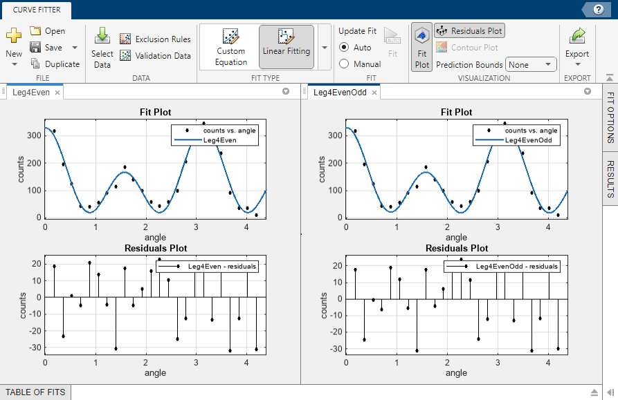
The fit appears to follow the trend of the data well, while the residuals appear to be randomly distributed and do not exhibit any systematic behavior.
Examine the numerical fit results in the Results pane. Look at each coefficient value and its confidence bounds in parentheses. The 95% confidence bounds indicate that the coefficients associated with a₀(x) and a₄(x) are known fairly accurately, but that the a₂(x) coefficient has a relatively large uncertainty.
To confirm the theoretical argument that the alpha-emission data is best described by a fourth-degree Legendre polynomial with only even terms, next fit the data using both even and odd terms:
$y_{2} (x) = y_{1} (x) + a_{1} x + a_{3} (\frac{1}{2}) (5 x^{3} - 3 x)$
First, make a copy of the Legendre polynomial fit to modify. On the Curve Fitter tab, in the File section, click Duplicate. The duplicated fit appears in a new tab in the Fits pane.
In the Table Of Fits pane, rename the new fit to Leg4EvenOdd.
In the Fit Options pane, change the equation terms.
Edit the terms as follows to fit the model given by y₂(x):
1. Click the last + button twice, to add the odd Legendre terms.
2. Change the new coefficient names to a1 and a3.
3. Change the Terms value for a1 to the following:
  cos(x)
4. Change the Terms value for a3 to the following:
  (1/2)*(5*cos(x)^3-3*cos(x))
Observe the new fit plotted in the Curve Fitter app, and examine the numerical results in the Results pane.
Note that the odd Legendre coefficients (a1 and a3) are likely candidates for removal to simplify the fit because their values are small and their confidence bounds contain zero. These results indicate that the odd Legendre terms do not contribute significantly to the fit, and the even Legendre terms are essentially unchanged from the previous fit. This confirms that the initial model choice in the Leg4Even fit is the best one.
Compare the fits side by side. Click the Document Actions button located to the far right of the fit figure tabs. Select the Tile All option and specify a 1-by-2 layout.
You can display only the plots by dragging and hiding the Fit Options, Results, and Table Of Fits panes.

Fit Custom Linear Legendre Polynomials at the Command Line

Fit the same model at the command line that you created in the Curve Fitter app.

To use a linear fitting algorithm, specify a cell array or string array of model terms as an input to the fittype function. Use the same Terms you entered in the Curve Fitter app for the Leg4Even fit, and do not specify any coefficients.
```
linearft = fittype({'(1/2)*(3*cos(x)^2-1)', ...
'(1/8)*(35*cos(x)^4-30*cos(x)^2+3)','1'})
```
```
linearft = 

     Linear model:
     linearft(a,b,c,x) = a*((1/2)*(3*cos(x)^2-1))...
       + b*((1/8)*(35*cos(x)^4-30*cos(x)^2+3)) + c
```
Load the angle and counts variables in the workspace.
```
load carbon12alpha
```

Use the fittype as an input to the fit function, and specify the angle and counts variables in the workspace.

f = fit(angle,counts,linearft)

f = 

     Linear model:
     f(x) = a*((1/2)*(3*cos(x)^2-1))...
     + b*((1/8)*(35*cos(x)^4-30*cos(x)^2+3)) + c
     Coefficients (with 95% confidence bounds):
       a =       23.86  (4.436, 43.29)
       b =       201.9  (180.2, 223.6)
       c =       102.9  (93.21, 112.5)

Plot the fit and data.
```
plot(f,angle,counts)
```

For more details on linear model terms, see the fittype function.