Avoid Obstacles Using Reinforcement Learning for Mobile Robots

Load Map

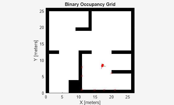
Load a map matrix, simpleMap, that represents the environment for the robot.

load exampleMaps simpleMap 
load exampleHelperOfficeAreaMap office_area_map
mapMatrix = simpleMap;
mapScale = 1;

Range Sensor Parameters

Next, set up a rangeSensor object which simulates a noisy range sensor. The range sensor readings are considered observations by the agent. Define the angular positions of the range readings, the max range, and the noise parameters.

scanAngles = -3*pi/8:pi/8:3*pi/8;
maxRange = 12;
lidarNoiseVariance = 0.1^2;
lidarNoiseSeeds = randi(intmax,size(scanAngles));

Robot Parameters

The action of the agent is a two-dimensional vector $$a=[v,\omega ]$$ where $$v$$ and $$\omega$$ are the linear and angular velocities of our robot. The DDPG agent uses normalized inputs for both the angular and linear velocities, meaning the actions of the agent are a scalar between -1 and 1, which is multiplied by the maxLinSpeed and maxAngSpeed parameters to get the actual control. Specify this maximum linear and angular velocity.

Also, specify the initial position of the robot as [x y theta].

% Max speed parameters
maxLinSpeed = 0.3;
maxAngSpeed = 0.3;

% Initial pose of the robot
initX = 17;
initY = 15;
initTheta = pi/2;

Show Map and Robot Positions

To visualize the actions of the robot, create a figure. Start by showing the occupancy map and plot the initial position of the robot.

fig = figure("Name","simpleMap");
set(fig, "Visible","on");
ax = axes(fig);

show(binaryOccupancyMap(mapMatrix),"Parent",ax);
hold on
plotTransforms([initX,initY,0],eul2quat([initTheta,0,0]),"MeshFilePath","groundvehicle.stl","View","2D");
light;
hold off

Environment Interface

Create an environment model that takes the action, and gives the observation and reward signals. Specify the provided example model name, exampleHelperAvoidObstaclesMobileRobot, the simulation time parameters, and the agent block name.

mdl = "exampleHelperAvoidObstaclesMobileRobot";
Tfinal = 100;
sampleTime = 0.1;

agentBlk = mdl + "/Agent";

Open the model.

open_system(mdl)

The model contains the Environment and Agent blocks. The Agent block is not defined yet.

Inside the Environment Subsystem block, you should see a model for simulating the robot and sensor data. The subsystem takes in the action, generates the observation signal based on the range sensor readings, and calculates the reward based on the distance from obstacles, and the effort of the action commands.

open_system(mdl + "/Environment")

Define observation parameters, obsInfo, using the rlNumericSpec object and giving the lower and upper limit for the range readings with enough elements for each angular position in the range sensor.

obsInfo = rlNumericSpec([numel(scanAngles) 1],...
    "LowerLimit",zeros(numel(scanAngles),1),...
    "UpperLimit",ones(numel(scanAngles),1)*maxRange);
numObservations = obsInfo.Dimension(1);

Define action parameters, actInfo. The action is the control command vector, $$a=[v,\omega ]$$, normalized to $$[-1,1]$$.

numActions = 2;
actInfo = rlNumericSpec([numActions 1],...
    "LowerLimit",-1,...
    "UpperLimit",1);

Build the environment interface object using rlSimulinkEnv (Reinforcement Learning Toolbox). Specify the model, agent block name, observation parameters, and action parameters. Set the reset function for the simulation using exampleHelperRLAvoidObstaclesResetFcn. This function restarts the simulation by placing the robot in a new random location to begin avoiding obstacles.

env = rlSimulinkEnv(mdl,agentBlk,obsInfo,actInfo);
env.ResetFcn = @(in)exampleHelperRLAvoidObstaclesResetFcn(in,scanAngles,maxRange,mapMatrix);
env.UseFastRestart = "Off";

For another example that sets up a Simulink® environment for training, see Create Simulink Environment and Train Agent (Reinforcement Learning Toolbox).

DDPG Agent

A DDPG agent approximates the long-term reward given observations and actions using a critic value function representation. To create the critic, first create a deep neural network with two inputs, the observation and action, and one output. For more information on creating a deep neural network value function representation, see Create Policies and Value Functions (Reinforcement Learning Toolbox).

statePath = [
    featureInputLayer(numObservations, "Normalization","none","Name","State")
    fullyConnectedLayer(50,"Name","CriticStateFC1")
    reluLayer("Name","CriticRelu1")
    fullyConnectedLayer(25,"Name","CriticStateFC2")];
actionPath = [
    featureInputLayer(numActions,"Normalization","none","Name","Action")
    fullyConnectedLayer(25,"Name","CriticActionFC1")];
commonPath = [
    additionLayer(2,"Name","add")
    reluLayer("Name","CriticCommonRelu")
    fullyConnectedLayer(1,"Name","CriticOutput")];

criticNetwork = layerGraph();
criticNetwork = addLayers(criticNetwork,statePath);
criticNetwork = addLayers(criticNetwork,actionPath);
criticNetwork = addLayers(criticNetwork,commonPath);
criticNetwork = connectLayers(criticNetwork,"CriticStateFC2","add/in1");
criticNetwork = connectLayers(criticNetwork,"CriticActionFC1","add/in2");
criticNetwork = dlnetwork(criticNetwork);

Next, specify options for the critic optimizer using rlOptimizerOptions.

Finally, create the critic representation using the specified deep neural network and options. You must also specify the action and observation specifications for the critic, which you obtain from the environment interface. For more information, see rlQValueFunction (Reinforcement Learning Toolbox).

criticOptions = rlOptimizerOptions("LearnRate",1e-3,"L2RegularizationFactor",1e-4,"GradientThreshold",1);
critic = rlQValueFunction(criticNetwork,obsInfo,actInfo,"ObservationInputNames","State","ActionInputNames","Action");

A DDPG agent decides which action to take given observations using an actor representation. To create the actor, first create a deep neural network with one input, the observation, and one output, the action.

Finally, construct the actor in a similar manner as the critic. For more information, see rlContinuousDeterministicActor (Reinforcement Learning Toolbox).

actorNetwork = [
    featureInputLayer(numObservations,"Normalization","none","Name","State")
    fullyConnectedLayer(50,"Name","actorFC1")
    reluLayer("Name","actorReLU1")
    fullyConnectedLayer(50, "Name","actorFC2")
    reluLayer("Name","actorReLU2")
    fullyConnectedLayer(2, "Name","actorFC3")
    tanhLayer("Name","Action")];
actorNetwork = dlnetwork(actorNetwork);

actorOptions = rlOptimizerOptions("LearnRate",1e-4,"L2RegularizationFactor",1e-4,"GradientThreshold",1);
actor = rlContinuousDeterministicActor(actorNetwork,obsInfo,actInfo);

Create DDPG agent object

Specify the agent options.

agentOpts = rlDDPGAgentOptions(...
    "SampleTime",sampleTime,...
    "ActorOptimizerOptions",actorOptions,...
    "CriticOptimizerOptions",criticOptions,...
    "DiscountFactor",0.995, ...
    "MiniBatchSize",128, ...
    "ExperienceBufferLength",1e6); 

agentOpts.NoiseOptions.Variance = 0.1;
agentOpts.NoiseOptions.VarianceDecayRate = 1e-5;

Create the rlDDPGAgent object. The obstacleAvoidanceAgent variable is used in the model for the Agent block.

obstacleAvoidanceAgent = rlDDPGAgent(actor,critic,agentOpts);
open_system(mdl + "/Agent")

Reward

The reward function for the agent is modeled as shown.

The agent is rewarded to avoid the nearest obstacle, which minimizes the worst-case scenario. Additionally, the agent is given a positive reward for higher linear speeds, and is given a negative reward for higher angular speeds. This rewarding strategy discourages the agent's behavior of going in circles. Tuning your rewards is key to properly training an agent, so your rewards vary depending on your application.

Train Agent

To train the agent, first specify the training options. For this example, use the following options:

For more information, see rlTrainingOptions (Reinforcement Learning Toolbox).

maxEpisodes = 10000;
maxSteps = ceil(Tfinal/sampleTime);
trainOpts = rlTrainingOptions(...
    "MaxEpisodes",maxEpisodes, ...
    "MaxStepsPerEpisode",maxSteps, ...
    "ScoreAveragingWindowLength",50, ...
    "StopTrainingCriteria","AverageReward", ...
    "StopTrainingValue",400, ...
    "Verbose", true, ...
    "Plots","training-progress");

Train the agent using the train (Reinforcement Learning Toolbox) function. Training is a computationally-intensive process that takes several minutes to complete. To save time while running this example, load a pretrained agent by setting doTraining to false. To train the agent yourself, set doTraining to true.

doTraining = false; % Toggle this to true for training. 

if doTraining
    % Train the agent.
    trainingStats = train(obstacleAvoidanceAgent,env,trainOpts);
else
    % Load pretrained agent for the example.
    load exampleHelperAvoidObstaclesAgent obstacleAvoidanceAgent
end

The Reinforcement Learning Episode Manager can be used to track episode-wise training progress. As the episode number increases, you want to see an increase in the reward value.

Simulate

Use the trained agent to simulate the robot driving in the map and avoiding obstacles for 200 seconds.

set_param("exampleHelperAvoidObstaclesMobileRobot","StopTime","200");
out = sim("exampleHelperAvoidObstaclesMobileRobot.slx");

Visualize

To visualize the simulation of the robot driving around the environment with range sensor readings, use the helper, exampleHelperAvoidObstaclesPosePlot.

for i = 1:5:size(out.range,3)
    u = out.pose(i,:);
    r = out.range(:,:,i);
    exampleHelperAvoidObstaclesPosePlot(u,mapMatrix,mapScale,r,scanAngles,ax);
end

Extensibility

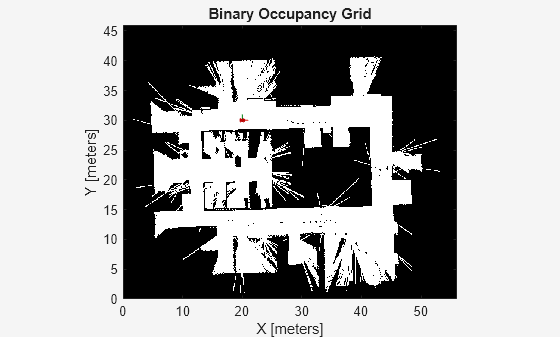
You can now use this agent to simulate driving in a different map. Another map generated from lidar scans of an office environment is used with the same trained model. This map represents a more realistic scenario to apply the trained model after training.

Change the map

mapMatrix = office_area_map.occupancyMatrix > 0.5;
mapScale = 10;
initX = 20;
initY = 30;
initTheta = 0;
fig = figure("Name","office_area_map");
set(fig,"Visible","on");
ax = axes(fig);
show(binaryOccupancyMap(mapMatrix,mapScale),"Parent",ax);
hold on
plotTransforms([initX,initY,0],eul2quat([initTheta, 0, 0]),"MeshFilePath","groundvehicle.stl","View","2D");
light;
hold off

Simulate

Simulate the robot's trajectory across the new map. Reset the simulation time in case the agent needs to be re-trained and retuned later.

out = sim("exampleHelperAvoidObstaclesMobileRobot.slx");
set_param("exampleHelperAvoidObstaclesMobileRobot","StopTime","inf");

Visualize

for i = 1:5:size(out.range,3)
    u = out.pose(i,:);
    r = out.range(:,:,i);
    exampleHelperAvoidObstaclesPosePlot(u,mapMatrix,mapScale,r,scanAngles,ax);
end